MRaster Color Schemes

1. Introduction
- 1.1. Color Scheme Class Interface
2. Color Cube Edge/Diagonal Graph Color Schemes
3. Continuous Polynomial Schemes
4. Dave Green's cubehelix color maps
5. Pseudo-Greyscale
6. Spectral
7. Color Brewer
8. Web Safe & Color Blind Pallets
9. Miscilanious Pallets
10. Binary Pallets
11. Predefined Color Scheme Cross Reference

1. Introduction

MRaster provides access to a rich collection of color schemes. Color schemes are exposed in the API as inner classes of the colorTpl class. These inner classes follow a regular naming convention:

csCB .......... RGB Color Brewer 2 (template: csCB_tpl
csFP .......... RGB Fixed pallets (template: csFP_tpl
csWS .......... RGB Web safe colors (template: csFP_tpl)
csCCdiag ...... RGB color cube: diagonal gradients (template: csCC_tpl)
csCCcons ...... RGB color cube: Gradients with constant brightness (template: csCC_tpl)
csCColde ...... RGB color cube: Some classic color gradients (template: csCC_tpl)
csCCud ........ RGB color cube: Two color up-down ramps (template: csCC_tpl)
csCCdiv ....... RGB color cube: Three Segment Diverging Maps (template: csCC_tpl)
csCCSum ....... RGB color cube: Sum ramp (template: csCC_tpl)
csCCu ......... RGB color cube: Gradients from black to another corner (template: csCC_tpl)
csCCwic ...... RGB color cube: White In Center Circular Gradients (template: csCC_tpl)
csCCfractal ... RGB color cube: Common gradient schemes used for fractals (template: csCC_tpl)
csHSLh ........ RGB color cube: Gradients from the cube center to a corner (template: csHSLh_tpl)
csBin ......... RGB Binary Schemes (template: csCC_tpl)
csPGrey ....... RGB Pseudo-greyscale
csRainbow ..... RGB spectrum based colors
csCH .......... RGB Cubehelix colors (template: csCubeHelix_tpl)
csBin ......... Defined by parametric polynomial curves in the RGB color cube. (template: csPLY_tpl)

These classes are static in nature, and an instance is not required to use them. They all have members named "c" which can set the color of an existing colorTpl instance (a "setter") or create a brand new instance (a "factory").

When used as a factory, color scheme classes return fully constructed colorTpl objects:

mjr:color3c8b aColor = mjr::color3c8b::webSafeNormalVision.c(25);

Alternately, color scheme classes may set the components of a passed colorTpl instance:

mjr::color3c8b aColor;
mjr::color3c8b::webSafeNormalVision.c(aColor, 25);

Color scheme classes may also be used by colorTpl methods to identify a color scheme. For example, the csSet method can set the current object's components based on a color scheme like so:

mjr::color3c8b aColor;
aColor.csSet<mjr::color3c8b::webSafeNormalVision>(25);

1.1. Color Scheme Class Interface

Not all color scheme classes have the same interface; however, the interfaces are uniformly designed:

numC: The number of colors available in the scheme
- Color schemes with a fixed number of colors at compile time have member numC
- Color schemes with the number of colors set at run time, will have a numC argument for the c methods.
  - These schemes have two members specifying the range for numC: minNumC & maxNumC.
c: methods are used to set colors
- The c methods come in pairs:
  - A colorTpl factory method and that takes one or more arguments identifying the color within the color scheme
    - The first argument is the color scheme selector used to select a color from the scheme:
      - csIntType csIdx: An integer "index" for discrete color schemes (like Colorbrewer schemes)
      - csFltType csX: A floating point value in [0, 1] used to select colors from continuous schemes (like gradients)
      - csNatType csVal: A csFltType or csIntType depending on the clrChanT. Used as described above.
      - colorTpl csCol: A color object to be converted to a color. See the csHSLh* schemes as an example.
      - typename csG: A generic color selector used in a template
    - The remaining arguments are generally used to specify some characteristic of the scheme itself. Examples:
      - A numC argument specifying the number of elements in a discrete scheme (like Colorbrewer schemes)
      - The rainbow color schemes based on "color match functions" an argument interpMethod specifying an interpolation method.
  - A method that takes a colorTpl as it's first argument, with the remaining arguments as in the factory method form of c.
- It is entirely possible that a color scheme object may have more than two c methods. For example, csCC* color schemes have a pair of c methods taking integer color selectors and another pair taking a floating point color selectors.

Many color schemes provide a number of colors that is a function of chanStepMax, which is directly related to the value of clrChanT. For integral clrChanT types, chanStepMax will be equal to maxChanVal. For floating point clrChanT types, chanStepMax will be equal to $2^{31}$.

2. Color Cube Edge/Diagonal Graph Color Schemes

The RGB Color Cube                                       _________________________
                                                  green / _____________________  /| yellow
                                                       / / ___________________/ / |
                                                      / / /| |               / /  |
                                                     / / / | |              / / . |
                                                    / / /| | |             / / /| |
                                                   / / / | | |            / / / | |
                                                  / / /  | | |     white / / /| | |
                                                 / /_/__________________/ / / | | |
                                                /________________________/ /  | | |
Vertexes and Center of the Cube:           cyan | ______________________ | |  | | |
Name     R     G     B     Abriv                | | |    | | |_________| | |__| | |
black    0.0   0.0   0.0   0                    | | |    | |___________| | |____| |
blue     0.0   0.0   1.0   b                    | | |   / / ___________| | |_  / / red
green    0.0   1.0   0.0   g                    | | |  / / /           | | |/ / /
red      1.0   0.0   0.0   r                    | | | / / /  black     | | | / /
yellow   1.0   1.0   0.0   y                    | | |/ / /             | | |/ /
cyan     0.0   1.0   1.0   c                    | | | / /              | | ' /
magenta  1.0   0.0   1.0   m                    | | |/_/_______________| |  /
white    1.0   1.0   1.0   w                    | |____________________| | /
grey50   0.5   0.5   0.5   h               blue |________________________|/ magenta

The RGB color cube is usually considered as part of the 3D Euclidean space $\mathbb{R}^3$ – that is $R$, $G$, & $B$ are real values in $I=[0, 1]$. This subset of $\mathbb{R}^3$ is frequently called the "unit cube" and denoted by $I^3$. A gradient in this context is a continuous curve, $c:I\rightarrow I^3$, from one point in the cube to another. In this way we define an infinite sequence of colors. The most popular gradients are straight lines connecting two colors together. The next most popular is a pairwise linear curve connecting several colors together – usually with each linear component the same length.

Digital images are most commonly represented with integer values for $R$, $G$, & $B$. Most commonly unsigned, 8-bit integers – $0.0$ mapping to $0$ and $1.0$ mapping to $255$. In this scenario one might think of the RGB color space as a discrete set of $16777216$ values, and color gradients as finite sequences of discrete "steps" from one discrete color value to another. For example, a linear gradient from "green" to "yellow" will have precisely $256$ unique steps when the color space is defined in terms of 8-bit, integer color channels. Note that a linear gradient from "green" to "magenta", across the diagonal of the cube, will also have $256$ color steps – one of the oddities of distance measurement the discrete RGB space! Lastly, note that if we had a gradient from "green" through "yellow" and ending at "red", we would have have $511$ distinct colors. So discreet RGB color spaces produce discreet gradients, and the number of colors in the gradient will differ depending on the points traversed.

The corners of the color cube are by far the most popular choices for gradient control points. In describing these gradients it is usefully to think about the corners and how we can connect them as a mathematical graph.

The edges of the cube taken with the corners as vertexes form a graph (referred to as "the cube edge graph" in this documentation). Every trail (a walk with unique edges) with $n$ edges generates a color scheme with $\mathrm{maxChanVal}\cdot n - 1$ unique colors. To make this scheme unique, we define the tree to have one of its end points the "start" of the scheme – so we can map the integers from $[0,\mathrm{maxChanVal}\cdot n]$ to unique colors.

Example:

"BCG" defines a trail starting at B (blue), moving to C (cyan) next, and ending at G (green). The color scheme has $0$ mapped to blue (the first vertex), $256$ mapped to cyan (the second vertex), and $511$ mapped to green (the final vertex). For values between two vertex points, we linearly interpolate between the two values.

If we expand the graph to also include edges between the diagonal points of each face (cyan to yellow for example), we have a larger graph with more options. This graph is referred to as "the face edge/diagonal graph" in this documentation.

Lastly, we can expand that graph by adding one vertex, called h, at the center of the cube with edges extending to each corner. This graph is referred to as "complete cube graph with center" in this documentation.

Every color scheme in this section can be created via the cmpRGBcornerDGradiant() method of colorTpl; however, many are also available as predefined color scheme objects. The color schemes provided by the csCC_tpl template provide a dual interface. One provides a discreet view of gradients (the c methods with csIdx arguments), and the other provides a continuous view of gradients (the c methods with csX arguments). When the colors use floating point channels, the discreet gradients have $2^{31}$ steps between corner colors.

2.1. Maximal circuits in the cube edge graph

This is one of the most commonly seen color schemes in scientific visualization. The color cube rainbow map is generated by the unique six segment (6 vertex) cycle in the face edge graph not involving white or black:

RYGCBMR – csCColdeRainbow

2.1.1. Predefined Schemes

csCColdeRainbow

2.2. Maximal circuits in the cube edge/diagonal graph

If we expand to the edge face/diagonal graph, then we have may more six segment cycles not involving white or black:

RBCGYMR
RBCMYGR
RBGCMYR
RBGCYMR
RBGYCMR
RBMCGYR
RBMCYGR
RBMYCGR
RGBCMYR
RGBCYMR
RGBMCYR
RGCBMYR
RGYCBMR
RMBGCYR
RMCBGYR

2.3. Hitting all the corners

A common request is for a cycle in the face edge graph that uses every corner color of the RGB cube. Not only do we have one, but 6 uniquely different ones – not counting rearrangements or reversals:

0BCGYWMR0
0BCWMRYG0
0BMRYWCG0
0BMWCGYR0
0GCBMWYR0
0GYWCBMR0

2.4. Large Trees

Another common request is for trees (so no color is used twice) starting at black and ending at white. Several trees exist of lengths of 7 and 5:

0BCGYRMW
0BMRYGCW
0GCBMRYW
0GYRMBCW
0RMBCGYW
0RYGCBMW
0BCGYW
0BMRYW
0GCBMW
0GYRMW
0RMBCW
0RYGCW

2.5. Black to White in Three Trees

The three segment trees from black to white are useful in that the intensity (sum of the components) is a monotone increasing function from zero up to three. One of them (0RYW) is often called the "fire ramp" as it ranges from black (flame base), up to yellow, then red, and finally to white hot.

0BCW – csCCsumBGR
0BMW – csCCsumBRG
0GCW – csCCsumGBR
0GYW – csCCsumGRB
0RMW – csCCsumRBG
0RYW – csCCsumRGB & csCColdeFireRamp

2.5.1. Predefined Schemes

csCCsumBGR
csCCsumBRG
csCCsumGBR
csCCsumGRB
csCCsumRBG
csCCsumRGB & csCColdeFireRamp

2.6. Black to Corner in One Trees

These minimal trees go from black to a corner of the cube – not much of a tree!! Still, they are exceedingly common in applications, and thus have predefined color schemes.

0W – csCCu0W
0R – csCCu0R
0B – csCCu0B
0G – csCCu0G
0C – csCCu0C
0M – csCCu0M
0Y – csCCu0Y

2.6.1. Predefined Schemes

csCCu0W
csCCu0R
csCCu0B
csCCu0G
csCCu0C
csCCu0M
csCCu0Y

2.7. White In Center Circular Gradients

These three node cycles start and end with a primary or secondary color, and have white in the center. They are usefull for highlighting one segment of a circular data set – for example highlighting a sector of angles on a circle. As such they find application in complex number argument plots.

RWR – csCCwicR
GWG – csCCwicG
BWB – csCCwicB
MWM – csCCwicM
YWY – csCCwicY
CWC – csCCwicC

2.7.1. Predefined Schemes

csCCwicR
csCCwicG
csCCwicB
csCCwicM
csCCwicY
csCCwicC

2.8. Luminance based color schemes

Luminance based color schemes defined as color gradients from the center of the in the HSL color space to an extreem vertex are quite popular. Many of the most popular luminance based color schemes in the HSL color space are also edge graphs in the RGB color cube! Of particular note, are the two segment trees from black to white in the RGB edge/diagonal graph – they are the same as the two segment graphs in the edges of the HSL hexcone from black to white!

0RW – H=000 – red edge of the HSL hexcone
0YW – H=060 – yellow edge of the HSL hexcone
0GW – H=120 – green edge of the HSL hexcone
0CW – H=180 – cyan edge of the HSL hexcone
0BW – H=240 – blue edge of the HSL hexcone
0MW – H=300 – magenta edge of the HSL hexcone

2.9. Hot Too Cold

A very common color map used to map data with ranges from cold up to hot is known as the "cold too hot ramp". This ramp provides colors from blue, up through green, and ends in red. It suffers from the same defects as the color cube rainbow; however, its use is so common that special support is provided via a named method.

BCGYR – csCColdeColdToHot

The traditional cold to hot ramp can be improved – this is my personal opinion. This new ramp still has the same problems the color cube rainbow has; however, it is more attractive. This one moves from white (ice), up to water (blue), and then up to red (hot) via yellow.

WCBYR – csCColdeIceToWaterToHot

2.9.1. Predefined Schemes

csCColdeColdToHot
csCColdeIceToWaterToHot

2.10. Common Fractal Color Graphs

These color schemes have no special cycle/tree/graph structure at all, but they are commonly used to color fractals. Common enough that I have included predefined schemes for them.

0RYBCW – csCCfractal0RYBCW
YR – csCCfractalYR
YB – csCCfractalYB

2.10.1. Predefined Schemes

csCCfractal0RYBCW: $color_lut_docs_csCCfractal0RYBCW_50.png$
csCCfractalYR: $color_lut_docs_csCCfractalYR_50.png$
csCCfractalYB: $color_lut_docs_csCCfractalYB_50.png$

2.11. Constant Intensity Cycles

Two cycles, with three edges each, exhibiting constant intensity for every color in the color scheme are genuinely useful. They have the advantage that they always render a "bright" color. The lower intensity version is best for projected media that don't do well with yellow.

CMY – csCCconsTwo – intensity == 2
BRG – csCCconsOne – intensity == 1

2.11.1. Predefined Schemes

csCCconsTwo
csCCconsOne

2.12. One Segment Diverging Maps

One edge trees in the face diagonal graph with a nearly constant intensity of 2 along the entire edge are useful for "diverging" or "bipolar" color schemes. By definition, such color schemes will never involve black or white.

While rarely used, the following maps are useful and suggested. None of them have the problems associated with the color cube rainbow.

YC – csCCudBr
YM – csCCudBg
MC – csCCudGr
MY – csCCudGb
CM – csCCudRg
CY – csCCudRb

The naming convention for the methods is not obvious. Take, for example, setRGBcmpUpDownRampBr. This is so named because of the computational algorithm used to compute the scheme: Blue up, red down, green constant (maxChanVal).

2.12.1. Predefined Schemes

csCCudBr
csCCudBg
csCCudGr
csCCudGb
csCCudRg
csCCudRb

2.13. Three Segment Diverging Maps

Some three edge trees utilizing very different colors for starting and terminal points can form very nice "divergent" color maps. Such maps can successfully illustrate variables with both positive and negative values or two mutually exclusive, opposing variables. Only two are directly supported via named methods (selected for attractiveness):

BWR – intensity between 1 and 3
CWM – intensity between 2 and 3

2.13.1. Predefined Schemes

csCCdivBWR
csCCdivCWM

2.14. Center point ramps (HSL schemes)

Color schemes defined as gradients from the center of the HSL color space to an extreme edge are mostly perceptually linear. These are also one segment trees in the complete cube graph with center. Recall that we call the vertex at the center of the cube "H" – for "Half way between everything". Using this new vertex, we have the following saturation based color schemes:

HR – csHSLhR
HG – csHSLhG
HB – csHSLhB
HC – csHSLhC
HY – csHSLhY
HM – csHSLhM

2.14.1. Predefined Schemes

csHSLhR
csHSLhG
csHSLhB
csHSLhC
csHSLhY
csHSLhM

2.15. Stacked HSL Schemes

The diagonal traversals (diagonal meaning through the center of the cube) are essentially two of the HSL saturation based schemes placed back to back. Aside from the black-white one, these can form effective divergent color schemes.

CR – csCCdiagCR
MG – csCCdiagMG
YB – csCCdiagYB
0W – csCCdiag01

2.15.1. Predefined Schemes

csCCdiagCR
csCCdiagMG
csCCdiagYB
csCCdiag01

3. Continuous Polynomial Schemes

These schemes are "continuous" in that they take a floating point value to select the color, and are derived from continuous polynomial curves in the RGB cube space. Many of them are very similar, but not necessarily identical, to color maps in popular use (with similar names). In particular, the maps here may not be as precise when it comes to things like monotonously of intensity. That said these look nice and I like easy to compute color maps that don't require fancy interpolating schemes.

csPLYgrey
csPLYquad
csPLYinferno
csPLYmagma
csPLYparula
csPLYplasma
csPLYturbo
csPLYviridis
csPLYcividis
csPLYhsvRB

4. Dave Green's cubehelix color maps

The csCubeHelix_tpl templte can geneate any of the cubehelix schemes, but colorTpl predefines three I particularly like:

csCHstd
csCHblu
csCHvio

5. Pseudo-Greyscale

These schemes are not true greyscale, but the colors are very close to grey. These schemes are discreet!

csPGrey3x
csPGrey4x

6. Spectral

These color schemes are based on the spectrum and color match functions. These aren't really suitable for visualization, but some interesting color schemes can be derived from them.

csRainbowLA
csRainbowCM with BUMP
csRainbowCM with LINEAR
csRainbowCM with FLOOR
csRainbowCM with CEILING
csRainbowCM with NEAREST

7. Color Brewer

The discreet schemes in this section are all from the colorbrewer2 collection:

Credit: Brewer, Cynthia A., 2022. http://www.colorbrewer.org2, 2022-07-30.

Most of these schemes can provide a variable number of steps from 3 up to what is illustrated in each color swatch below. Also note that colorTpl provides a continuous gradient version of each color scheme – which is kinda weird, but I like some of them.

csCBAccent (3-8): 03
--
04
--
05
--
06
--
07
--
08
--
csCBBlues (3-9): 03
--
04
--
05
--
06
--
07
--
08
--
09
--
csCBBrBG (3-11): 03
--
04
--
05
--
06
--
07
--
08
--
09
--
10
--
11
--
csCBBuGn (3-9): 03
--
04
--
05
--
06
--
07
--
08
--
09
--
csCBBuPu (3-9): 03
--
04
--
05
--
06
--
07
--
08
--
09
--
csCBDark2 (3-8): 03
--
04
--
05
--
06
--
07
--
08
--
csCBGnBu (3-9): 03
--
04
--
05
--
06
--
07
--
08
--
09
--
csCBGreens (3-9): 03
--
04
--
05
--
06
--
07
--
08
--
09
--
csCBGreys (3-9): 03
--
04
--
05
--
06
--
07
--
08
--
09
--
csCBOranges (3-9): 03
--
04
--
05
--
06
--
07
--
08
--
09
--
csCBOrRd (3-9): 03
--
04
--
05
--
06
--
07
--
08
--
09
--
csCBPaired (3-12): 03
--
04
--
05
--
06
--
07
--
08
--
09
--
10
--
11
--
12
--
csCBPastel1 (3-9): 03
--
04
--
05
--
06
--
07
--
08
--
09
--
csCBPastel2 (3-9): 03
--
04
--
05
--
06
--
07
--
08
--
09
--
csCBPiYG (3-11): 03
--
04
--
05
--
06
--
07
--
08
--
09
--
10
--
11
--
csCBPRGn (3-11): 03
--
04
--
05
--
06
--
07
--
08
--
09
--
10
--
11
--
csCBPuBuGn (3-9): 03
--
04
--
05
--
06
--
07
--
08
--
09
--
csCBPuBu (3-9): 03
--
04
--
05
--
06
--
07
--
08
--
09
--
csCBPuOr (3-11): 03
--
04
--
05
--
06
--
07
--
08
--
09
--
10
--
11
--
csCBPuRd (3-9): 03
--
04
--
05
--
06
--
07
--
08
--
09
--
csCBPurples (3-9): 03
--
04
--
05
--
06
--
07
--
08
--
09
--
csCBRdBu (3-11): 03
--
04
--
05
--
06
--
07
--
08
--
09
--
10
--
11
--
csCBRdGy (3-11): 03
--
04
--
05
--
06
--
07
--
08
--
09
--
10
--
11
--
csCBRdPu (3-9): 03
--
04
--
05
--
06
--
07
--
08
--
09
--
csCBRdYlBu (3-11): 03
--
04
--
05
--
06
--
07
--
08
--
09
--
10
--
11
--
csCBRdYlGn (3-11): 03
--
04
--
05
--
06
--
07
--
08
--
09
--
10
--
11
--
csCBReds (3-9): 03
--
04
--
05
--
06
--
07
--
08
--
09
--
csCBSet1 (3-9): 03
--
04
--
05
--
06
--
07
--
08
--
09
--
csCBSet2 (3-8): 03
--
04
--
05
--
06
--
07
--
08
--
csCBSet3 (3-12): 03
--
04
--
05
--
06
--
07
--
08
--
09
--
10
--
11
--
12
--
csCBSpectral (3-11): 03
--
04
--
05
--
06
--
07
--
08
--
09
--
10
--
11
--
csCBYlGnBu (3-9): 03
--
04
--
05
--
06
--
07
--
08
--
09
--
csCBYlGn (3-9): 03
--
04
--
05
--
06
--
07
--
08
--
09
--
csCBYlOrBr (3-9): 03
--
04
--
05
--
06
--
07
--
08
--
09
--
csCBYlOrRd (3-8): 03
--
04
--
05
--
06
--
07
--
08
--

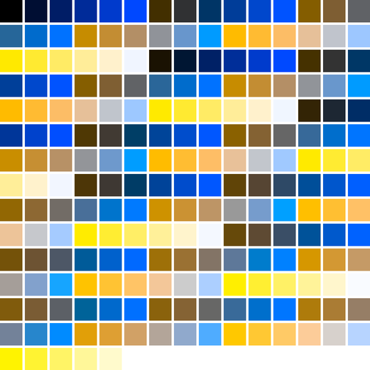
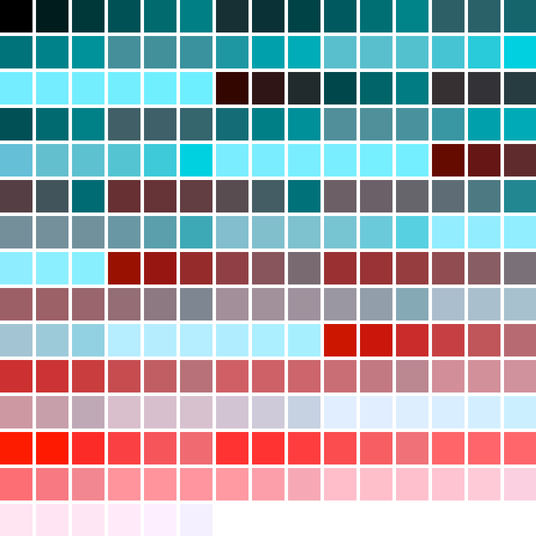
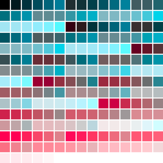
8. Web Safe & Color Blind Pallets

csWSSafeDeutanopia
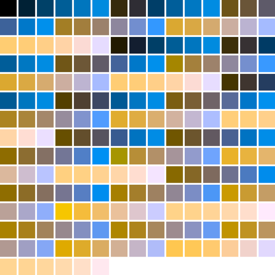
csWSSafeDeutanopiaAlt
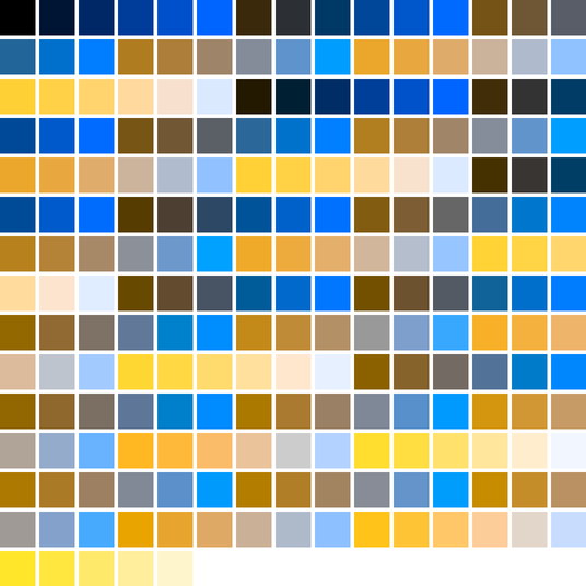
csWSSafeNormalVision
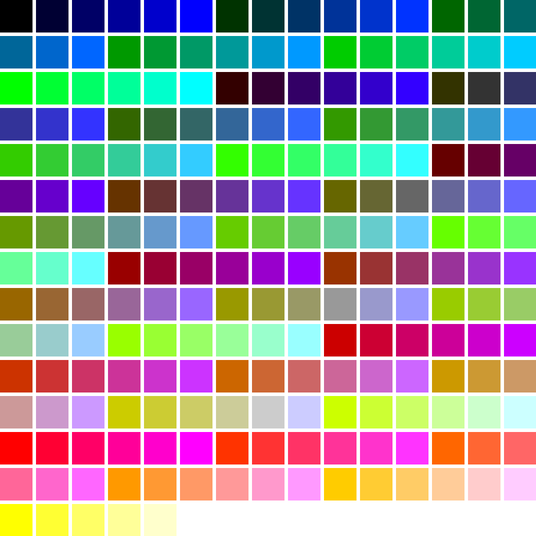
csWSSafeProtanopia
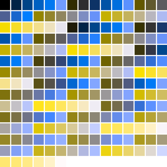
csWSSafeProtanopiaAlt
csWSSafeTritanoptia
csWSSafeTritanoptiaAlt

9. Miscilanious Pallets

These pallets are taken from various sources. Many of them are aviable in the NCAR collection of color maps. In some cases I have modified these maps from the origonal sources.

csFPblAqGrYeOrReVi200
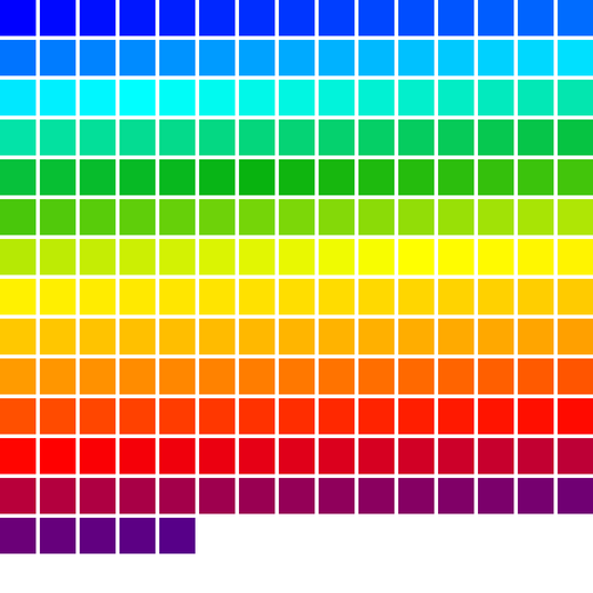
csFPcircular12
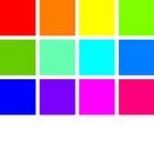
csFPcircular24
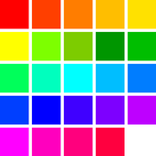
csFPcmoceanAlgae
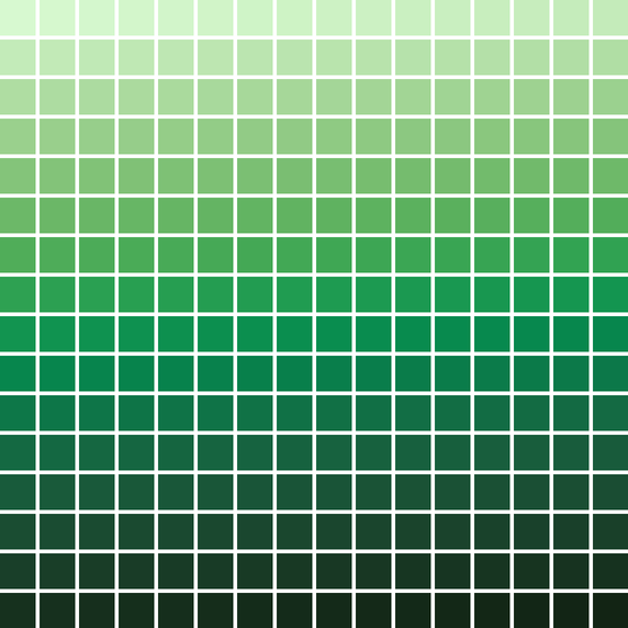
csFPcmoceanAmp
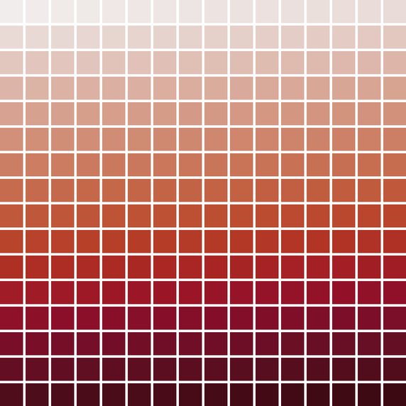
csFPcmoceanBalance
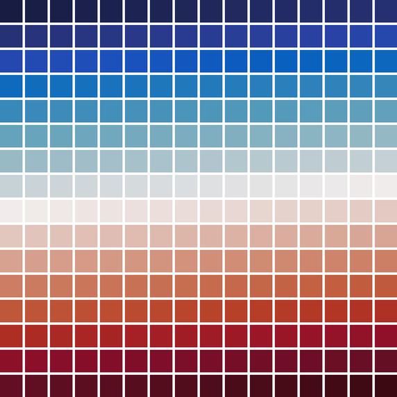
csFPcmoceanCurl
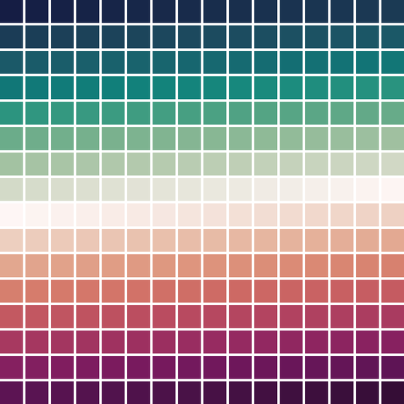
csFPcmoceanDeep
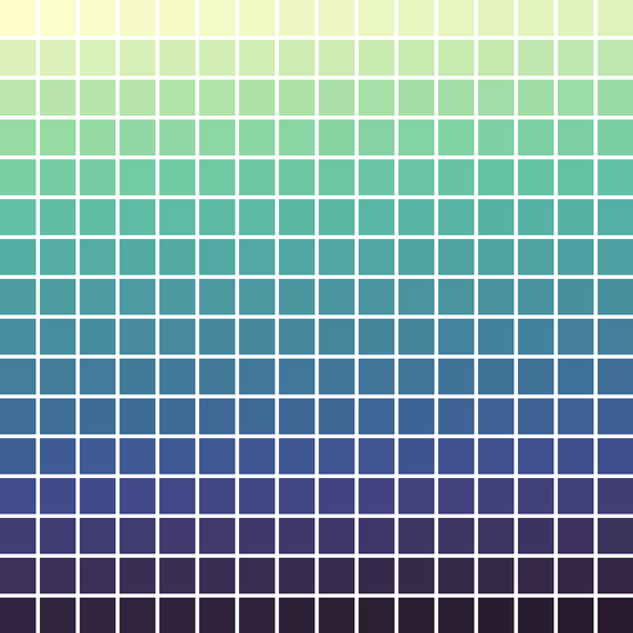
csFPcmoceanDense
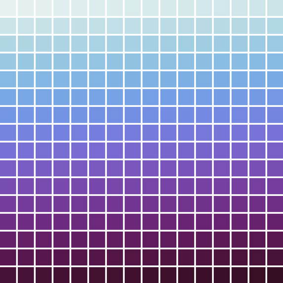
csFPcmoceanHaline
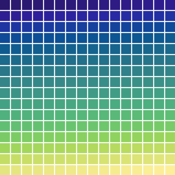
csFPcmoceanIce
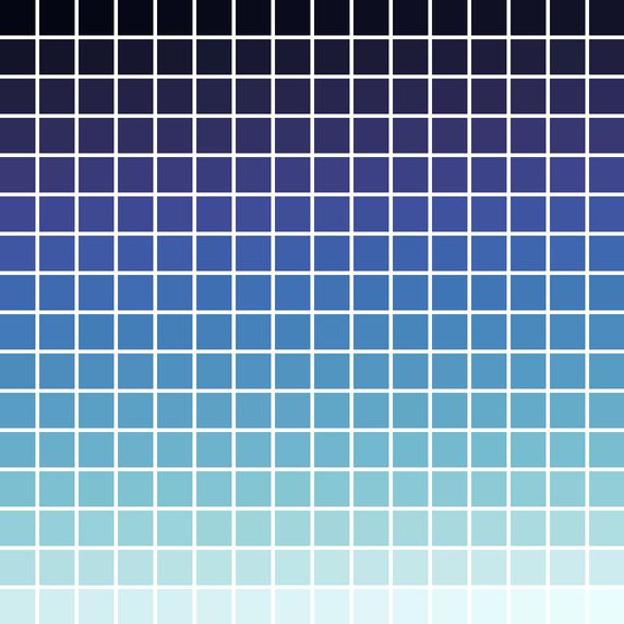
csFPcmoceanTempo
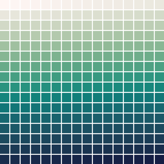
csFPmplBrBG
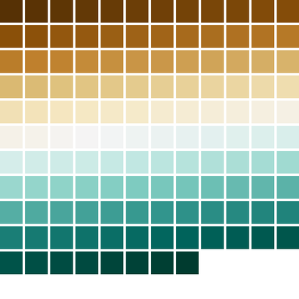
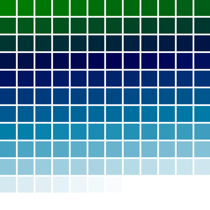
csFPmplOcean
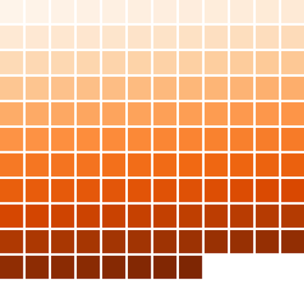
csFPmplOranges
csFPneoDdivVegetationA
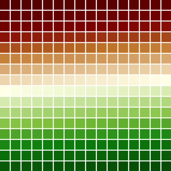
csFPneoDivVegetationC
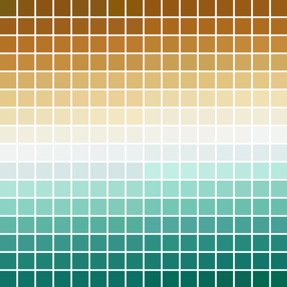
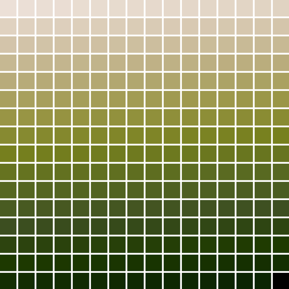
csFPneoModisNdvi

10. Binary Pallets

These are really just two color fixed pallets; however, they are generally used as infinite pallets that take on the first color for even indexes and the second color for odd indexes. Unlike fixed pallets, these do not have a "continuous" option and they are restricted to RGB corner colors.