Fortran Finance
Monte Carlo Simulation
| Author: | Mitch Richling |
| Updated: | 2025-11-06 09:21:32 |
| Generated: | 2025-11-06 09:21:33 |
Copyright © 2025 Mitch Richling. All rights reserved.
Table of Contents
These examples both use simple, resampling monte carlo on historical US financial data. Both examples include both Fortran code to run the simulations, and R code to visualize them. One of the examples illustrates endpoint distribution forecasting while the other illustrates trajectory forecasting.
1. inflation.f90 & inflation.R
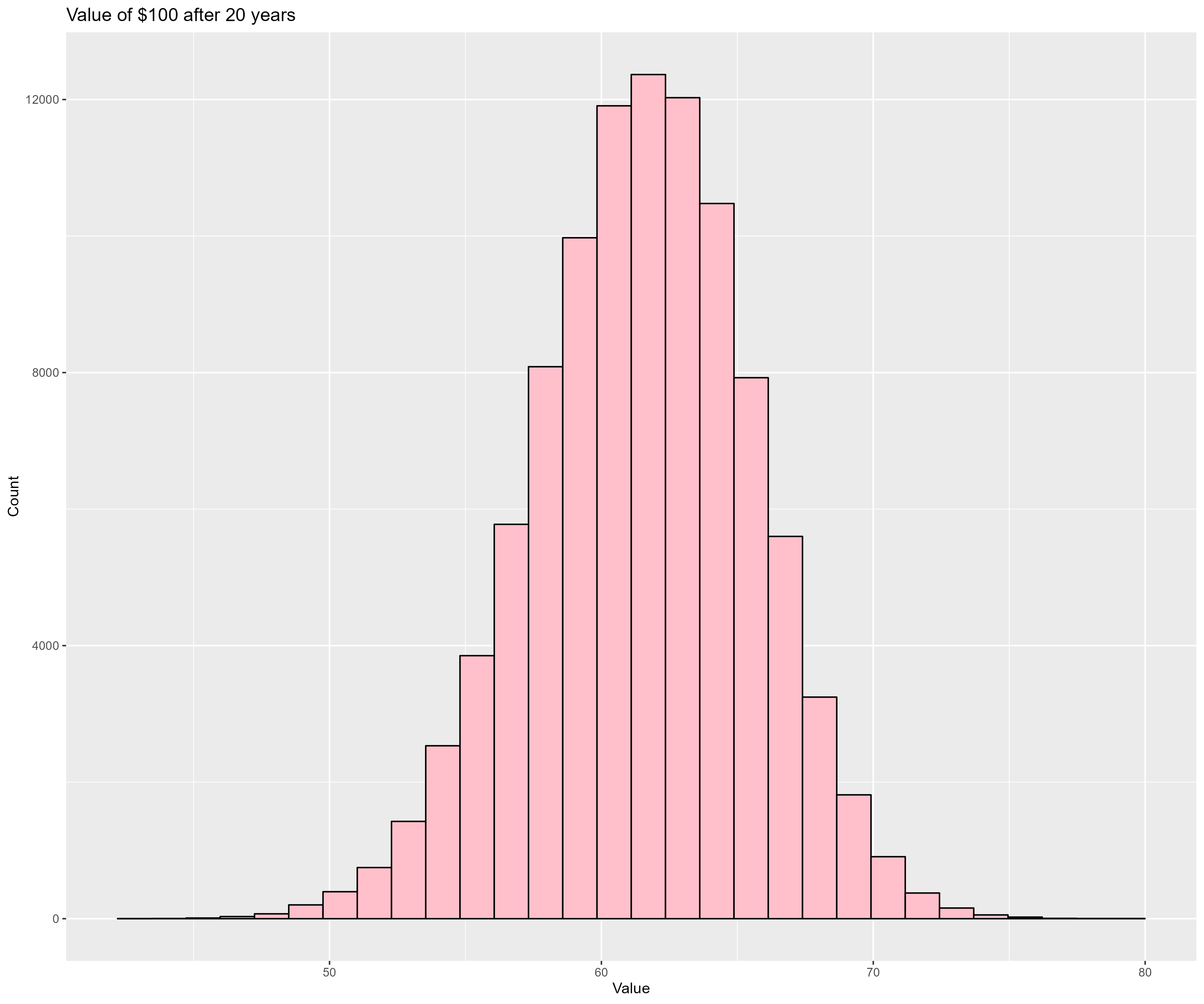
This program runs 100000 (tirals) Monte Carlo simulations of inflation for $100 (initial_value) over 20 (years) years
using the last 30 (mc_history_years) years of historical US inflation data. This program prints the value after 20 years
for each simulation to STDOUT. If placed in a file, this data may be consumed by inflation.R to produce a nice histogram
showing the probability of the value after 100 years.
Here is the Fortran code (inflation.f90):
program inflation
  use :: mrffl_config,       only: rk
  use :: mrffl_us_inflation, only: inf_resample

  implicit none (type, external)

  integer,          parameter :: years            = 20      ! Number of years to project out our inflation adjusted value
  integer,          parameter :: mc_history_years = 30      ! Number of years of US inflation data for our random inflation values
  integer,          parameter :: trials           = 100000  ! Number of trials to run
  real(kind=rk),    parameter :: initial_value    = 100     ! This is the value we will inflation adjusted over the years

  real(kind=rk)               :: value
  real(kind=rk)               :: i
  integer                     :: year, trial

  ! Run monte carlo simulations and dump the results to STDOUT
  print *, "trial value"
  do trial=1,trials
     value = initial_value
     do year=2,years
        i =  inf_resample(mc_history_years)
        value = value * (1 - i/100)
     end do
     print *, trial, value
  end do

end program inflation
And here is the R code (inflation.R):
source('../setup.R')

daDat <- fread("inflation.txt")

gp <- ggplot(data=daDat) +
  geom_histogram(aes(x=value), bins=30, col='black', fill='pink') +
  labs(title='Value of $100 after 20 years', x='Value', y='Count')

fname <- "inflation.png"
ggsave(fname, width=12, height=10)
if (is.character(imageV)) system(paste(imageV, fname, sep=' '))
2. stocks.f90 & stocks.R
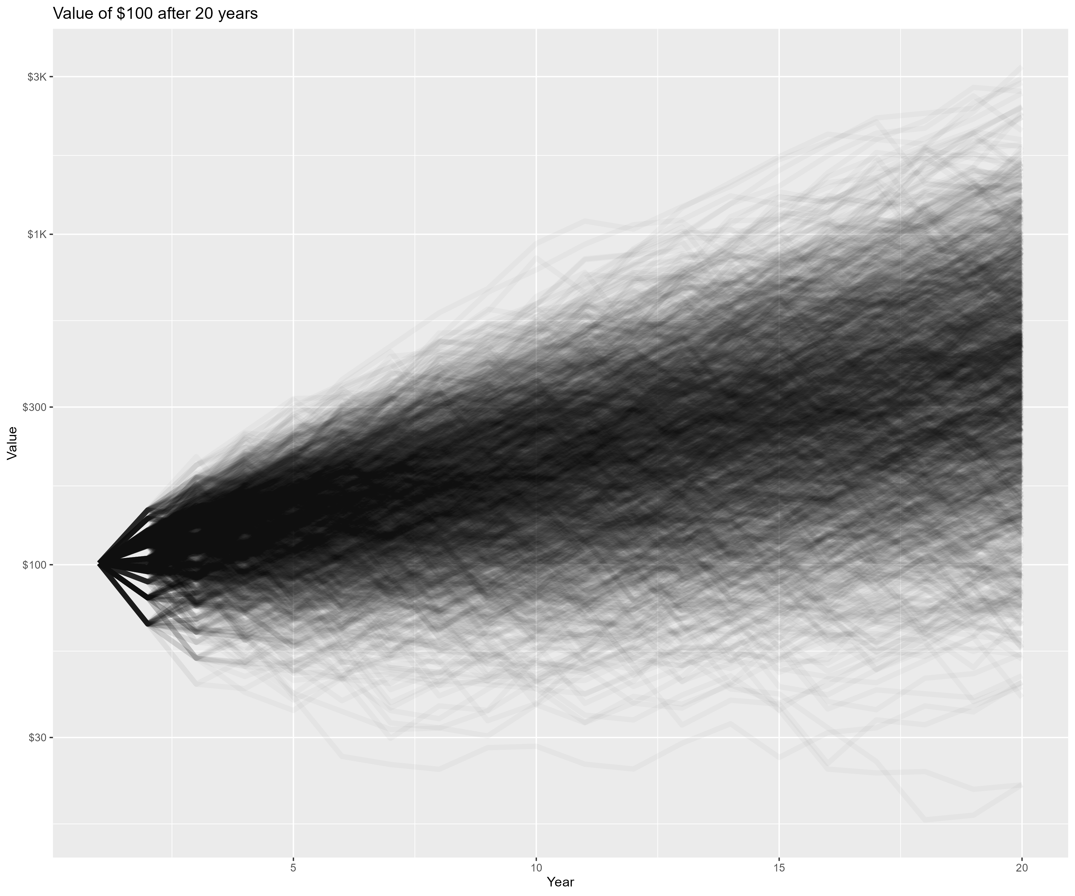
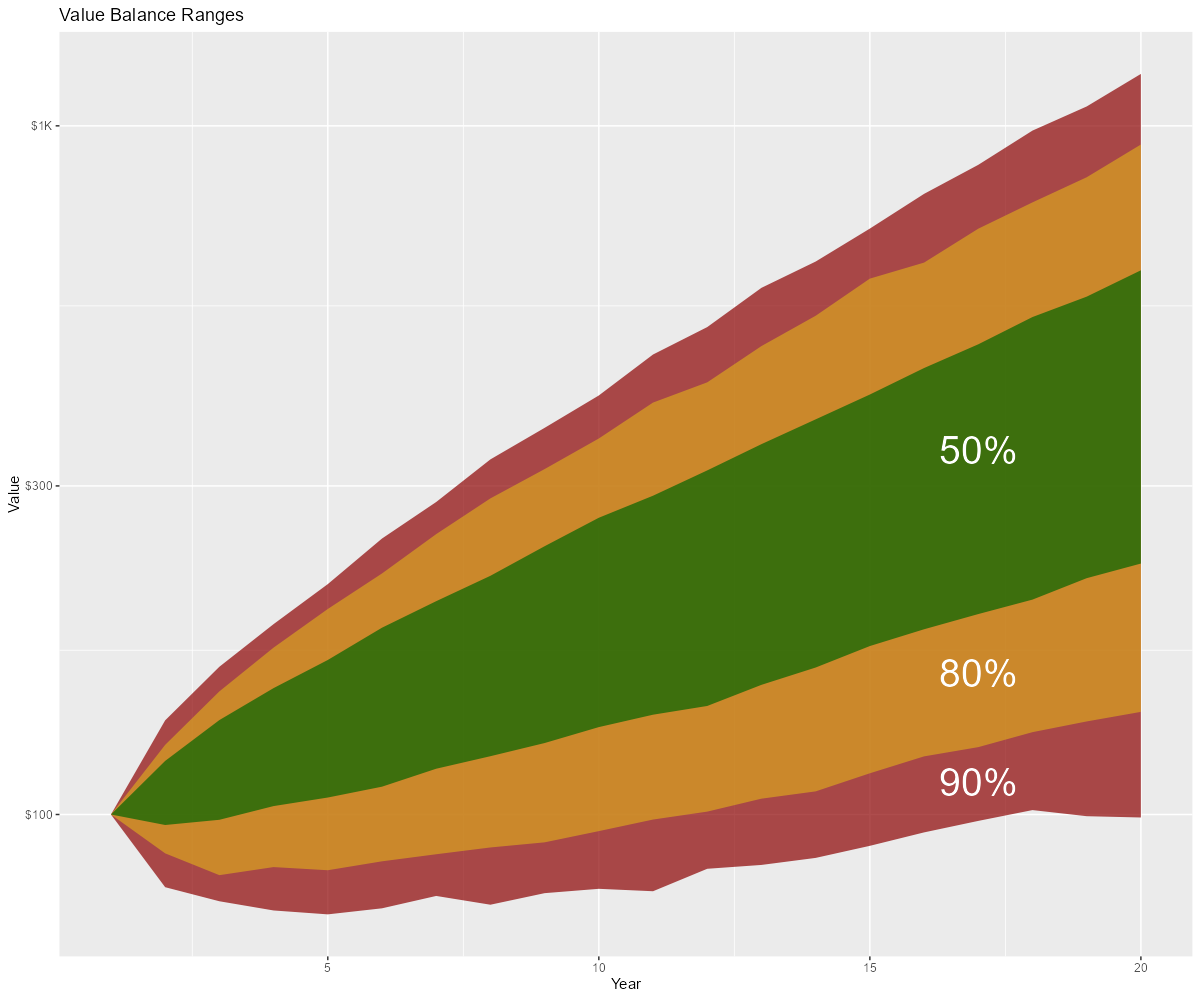
This program runs 2000 (trials) stocks simulations on $100 (initial_value). Each simulation is over 20 (years) years
using the last 30 (mc_history_years) years of historical US stocks data. This program prints the resulting value of each
simulation to STDOUT. If placed in a file, this data may be consumed by stocks.R to produce a nice histogram showing the
probability of the value after 100 years.
Here is the Fortran code (stocks.f90):
program stocks
  use :: mrffl_config,      only: rk
  use :: mrffl_us_markets,  only: rut_resample
  use :: mrffl_percentages, only: add_percentage

  implicit none (type, external)

  integer,          parameter :: years            = 20      ! Number of years to project out our stocks adjusted value
  integer,          parameter :: mc_history_years = 30      ! Number of years of US stocks data for our random stocks values
  integer,          parameter :: trials           = 2000    ! Number of trials to run
  real(kind=rk),    parameter :: initial_value    = 100     ! This is the value we will stocks adjusted over the years

  real(kind=rk)               :: value
  real(kind=rk)               :: i
  integer                     :: year, trial

  ! Run monte carlo simulations and dump the results to STDOUT
  print *, "trial year value"
  do trial=1,trials
     value = initial_value
     print *, trial, 1, value
     do year=2,years
        i =  rut_resample(mc_history_years)
        value = add_percentage(value, i)
        print *, trial, year, value
     end do
  end do

end program stocks
And here is the R code (stocks.R):
source('../setup.R')

daDat <- fread("stocks.txt") %>% mutate(trial=factor(trial))

gp <- ggplot(data=daDat) +
  geom_line(aes(x=year, y=value+1, group=trial), alpha=0.03, linewidth=2, col='black', show.legend=FALSE) +
  scale_y_continuous(labels = scales::label_dollar(scale_cut = cut_short_scale()), trans='log10') +
  labs(title='Value of $100 after 20 years', x='Year', y='Value')

fname <- "stocks_paths.png"
ggsave(fname, width=12, height=10)
if (is.character(imageV)) system(paste(imageV, fname, sep=' '))

bands <- c(90, 80, 50)

sumDat <- group_by(daDat, year) %>%
  summarize(band_90_0 = pmax(0, quantile(value,  (50-bands[1]/2)/100)),
            band_90_1 = pmax(0, quantile(value,  (50+bands[1]/2)/100)),
            band_80_0 = pmax(0, quantile(value,  (50-bands[2]/2)/100)),
            band_80_1 = pmax(0, quantile(value,  (50+bands[2]/2)/100)),
            band_50_0 = pmax(0, quantile(value,  (50-bands[3]/2)/100)),
            band_50_1 = pmax(0, quantile(value,  (50+bands[3]/2)/100)),
            .groups='keep')

gp <- ggplot(sumDat) +
  geom_ribbon(aes(x=year, ymin=band_90_0, ymax=band_90_1), fill='darkred',   alpha=0.7) +
  geom_ribbon(aes(x=year, ymin=band_80_0, ymax=band_80_1), fill='goldenrod', alpha=0.7) +
  geom_ribbon(aes(x=year, ymin=band_50_0, ymax=band_50_1), fill='darkgreen', alpha=0.7) +
  annotate("text", x=17, y=mean(c(sumDat$band_90_0[17], sumDat$band_80_0[17])), label="90%", col='white', size=10, vjust=0.5) +
  annotate("text", x=17, y=mean(c(sumDat$band_80_0[17], sumDat$band_50_0[17])), label="80%", col='white', size=10, vjust=0.5) +
  annotate("text", x=17, y=mean(c(sumDat$band_50_0[17], sumDat$band_50_1[17])), label="50%", col='white', size=10, vjust=0.5) +
  scale_y_continuous(labels = scales::label_dollar(scale_cut = cut_short_scale()), trans='log10') +
  labs(title='Value Balance Ranges') +
  ylab('Value') +
  xlab('Year')
fname <- 'stocks_ranges.png'
ggsave(fname, width=12, height=10, dpi=100, units='in', plot=gp);
if (is.character(imageV)) system(paste(imageV, fname, sep=' '))
3. blend_risk.f90 & blend_risk.R
Scenario:
We start with 4M in the bank. Over the next 50 years we wish to withdrawal 100K at the end of each year – and grow that value over time with inflation. We invest the money in a blend of S&P 500 and US 10 year treasury bonds.
Approach:
For each possible integer percentage mix of S&P & bonds (i.e. percentages of S&P that range from 0% up to 100%) we run 100000
(trials) simulations. The simulations use historical data. The technique is called "coupled resampling" where we pick a
random year, and use the measured values for that year for all three variables (S&P 500 return, 10 year US Treasury bond
return, and US inflation). This technique attempts to capture the inherent correlation between the variables; however, when
used with low resolution data it can create bias in the results. Note we can switch to uncoupled via the variable
coupled_mc.
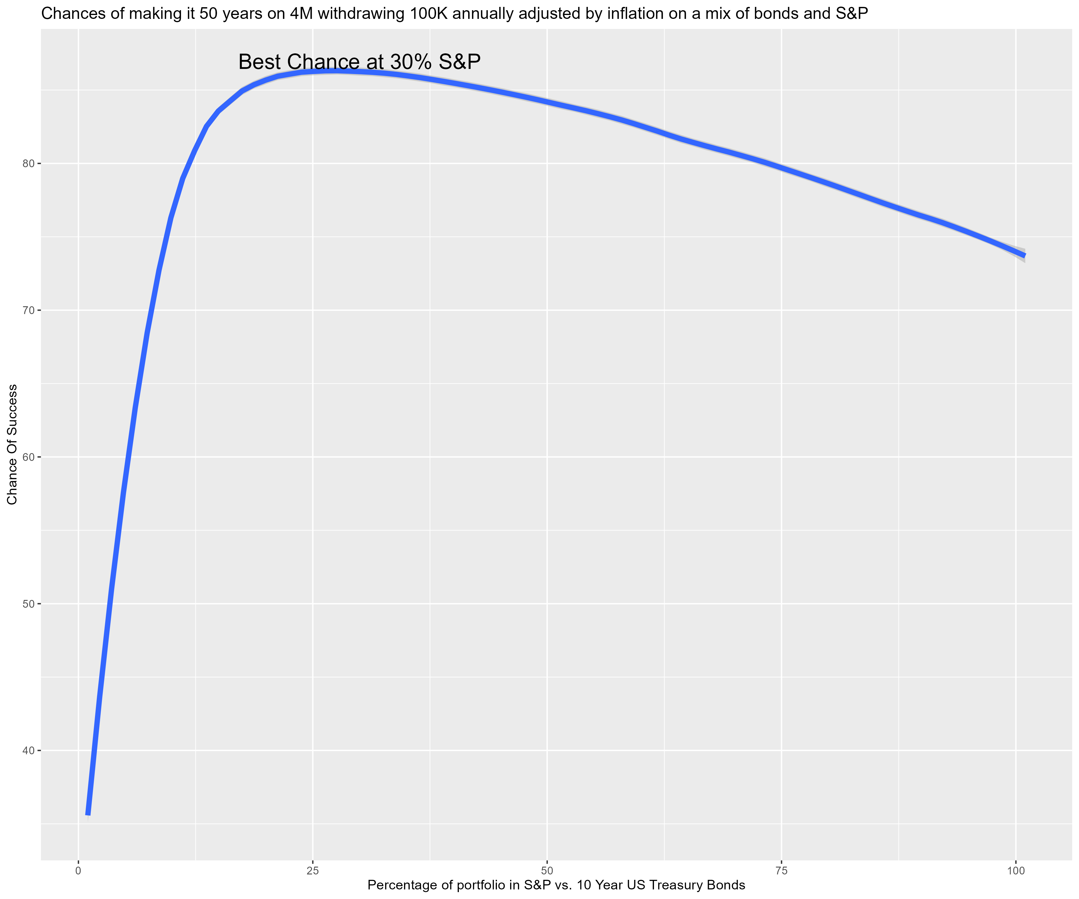
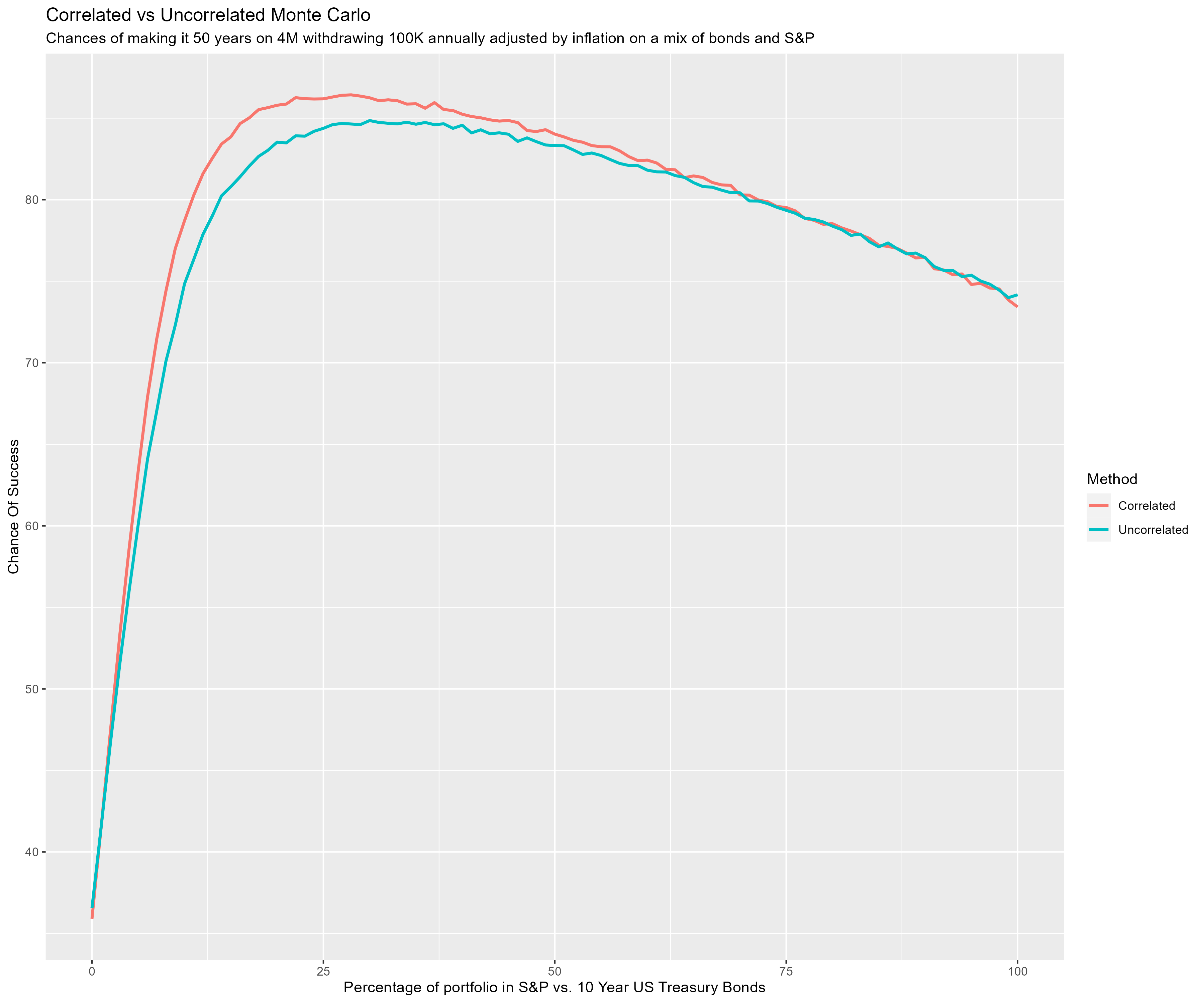
This next image shows the difference in results between coupled resampling (correlated) and uncoupled resampling (uncorrelated) monte carlo for this particular scenario.
Here is the Fortran code (blend_risk.f90):
program blend_risk
  use, intrinsic :: iso_fortran_env,    only: output_unit, error_unit
  use            :: mrffl_config,       only: rk
  use            :: mrffl_us_markets,   only: snp_dat, dgs10_dat
  use            :: mrffl_stats,        only: rand_int
  use            :: mrffl_us_inflation, only: inf_dat
  use            :: mrffl_percentages,  only: p_add=>add_percentage, p_of=>percentage_of

  implicit none (type, external)

  integer,          parameter :: years              = 50       ! Number of years to project out our stocks adjusted value
  integer,          parameter :: trials             = 100000   ! Number of trials to run
  real(kind=rk),    parameter :: initial_balance    = 4000000  ! This is the balance we will stocks adjusted over the years
  real(kind=rk),    parameter :: initial_withdrawal = 100000   ! Annual withdrawal
  logical,          parameter :: coupled_mc         = .TRUE.   ! Use coupled resampling

  real(kind=rk)               :: balance, withdrawal, c_snp, c_dgs, c_inf
  integer                     :: year, trial, hp
  integer                     :: rand_year

  ! Run monte carlo simulations and dump the results to STDOUT
  write (output_unit, '(a10,a10,a20)') "trial", "hp", "balance"
  do hp=0,100
     write (error_unit, '(a6,i0)') "hp=", hp
     do trial=1,trials
        balance = initial_balance
        withdrawal = initial_withdrawal
        do year=1,years
           if (coupled_mc) then
              rand_year = rand_int(2023, 2000)
              c_snp = snp_dat(rand_year)
              c_dgs = dgs10_dat(rand_year)
              c_inf = inf_dat(rand_year)
           else
              c_snp = snp_dat(rand_int(2023, 2000))
              c_dgs = dgs10_dat(rand_int(2023, 2000))
              c_inf = inf_dat(rand_int(2023, 2000))
           end if
           balance = p_add(p_of(balance, real(hp, rk)), c_snp) + p_add(p_of(balance, real(100-hp, rk)), c_dgs)
           balance = balance - min(withdrawal, balance)
           withdrawal = p_add(withdrawal, max(0.0_rk, c_inf))
        end do
        write (output_unit, '(i10,i10,f20.5)') trial, hp, balance
     end do
  end do

end program blend_risk
And here is the R code (blend_risk.R):
source('../setup.R')

daDat <- fread("blend_risk.txt") %>% mutate(hp=factor(hp))

## gp <- ggplot(data=daDat %>% filter(hp==75 & balance < 70e6)) +
##   geom_histogram(aes(x=balance), col='red', fill='pink', breaks=seq(0, 40e6, by=5e6)) +
##   scale_x_continuous(labels = scales::label_dollar(scale_cut = cut_short_scale())) +
##   labs(title='Ending balance of making it 50 years on 4M withdrawing 100K annually adjusted by inflation', x='Balance', y='')
## print(gp)

successDat <- daDat %>% group_by(hp) %>% summarize(success=100-100*sum(balance<=0)/length(balance), .groups='drop') %>% mutate(hp=as.integer(hp))

gp <- ggplot(data=successDat) +
  geom_smooth(aes(x=hp, y=success), method="loess", formula='y~x', span=0.2, level=.9999, se=TRUE, linewidth=2) +
  geom_text(data=successDat %>% filter(success == max(success)), aes(x=hp, y=success, label=paste('Best Chance at ', hp, '% S&P', sep='')), vjust='bottom', hjust='centered', size=6) +
  labs(title='Chances of making it 50 years on 4M withdrawing 100K annually adjusted by inflation on a mix of bonds and S&P', x='Percentage of portfolio in S&P vs. 10 Year US Treasury Bonds', y='Chance Of Success')

fname <- "blend_risk.png"
ggsave(fname, width=12, height=10)
if (is.character(imageV)) system(paste(imageV, fname, sep=' '))