Function Visualization

Author:	Mitch Richling
Updated:	2024-09-17 14:34:17
Generated:	2024-09-18 12:49:50

1. Introduction
2. Core Examples
3. Extra Examples

1. Introduction

In this document we break the process of mathematical function visualization into three steps:

Sample: The goal is to evaluate the function at various sample points so that we can faithfully approximate the geometric structure we are interested in visualizing. In the examples here, this step is almost entirely accomplished via the MR_rect_tree class. When possible we use more samples where the function behaviour is complex and fewer elseware.
Approximate: In this step we transform our sample data into a finite collection of geometric primitives (a "mesh" or a "cell complex") that may be visualized. In the examples here, this step is accomplished by the MR_cell_cplx and MR_rt_to_cc classes.
Explore: Finally we use Paraview to display & explore the data.

In some cases we preform post processing or use other tools: VisIT, meshlab, POV-Ray, Blender, ffmpeg, ImageMagick, etc…

2. Core Examples

This group of examples illistrate most of the features of MRPTree.

2.1. Complex Magnitude Surface Plot

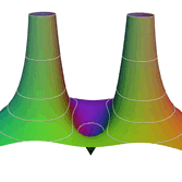
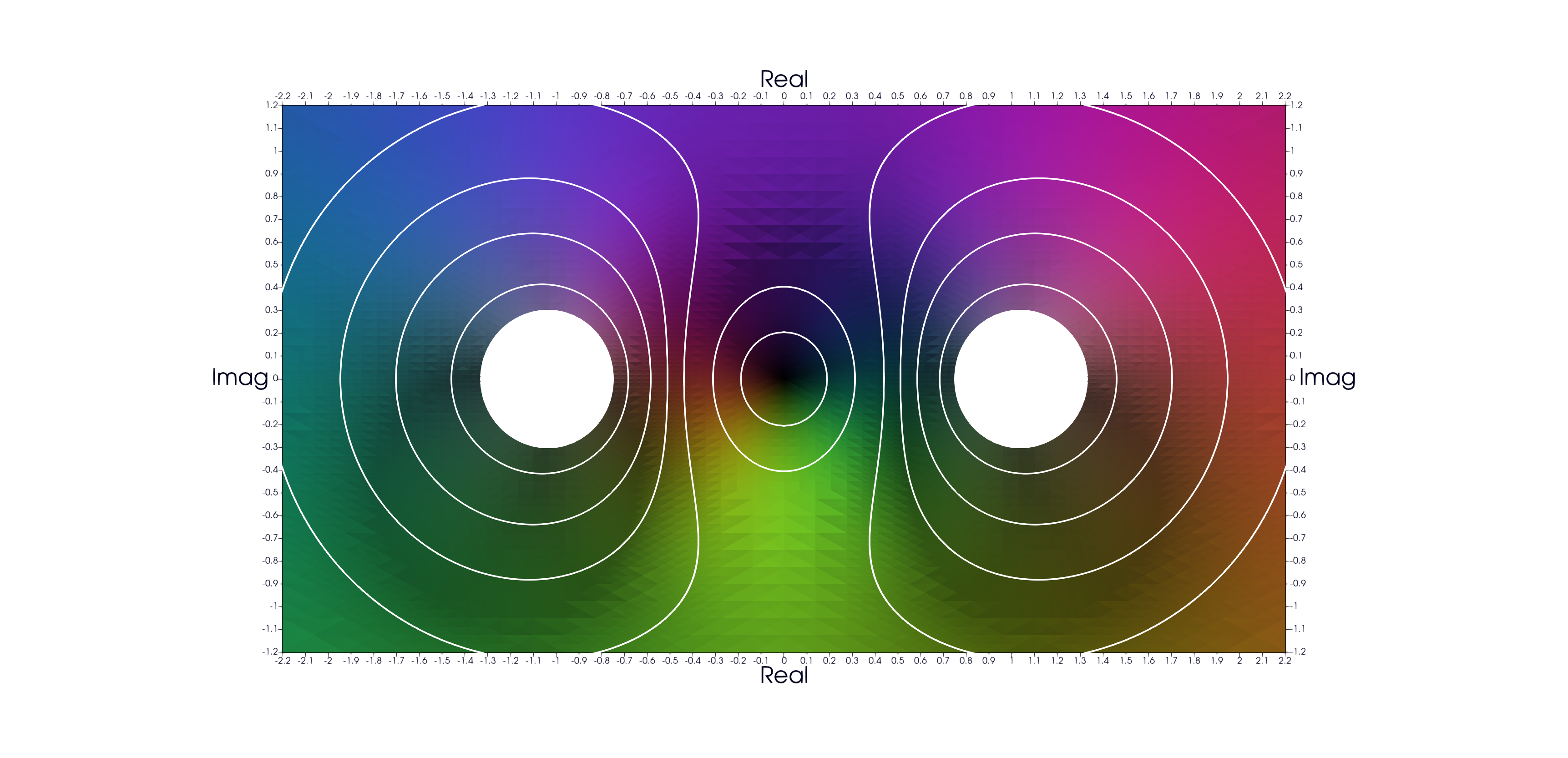
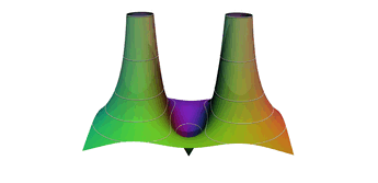
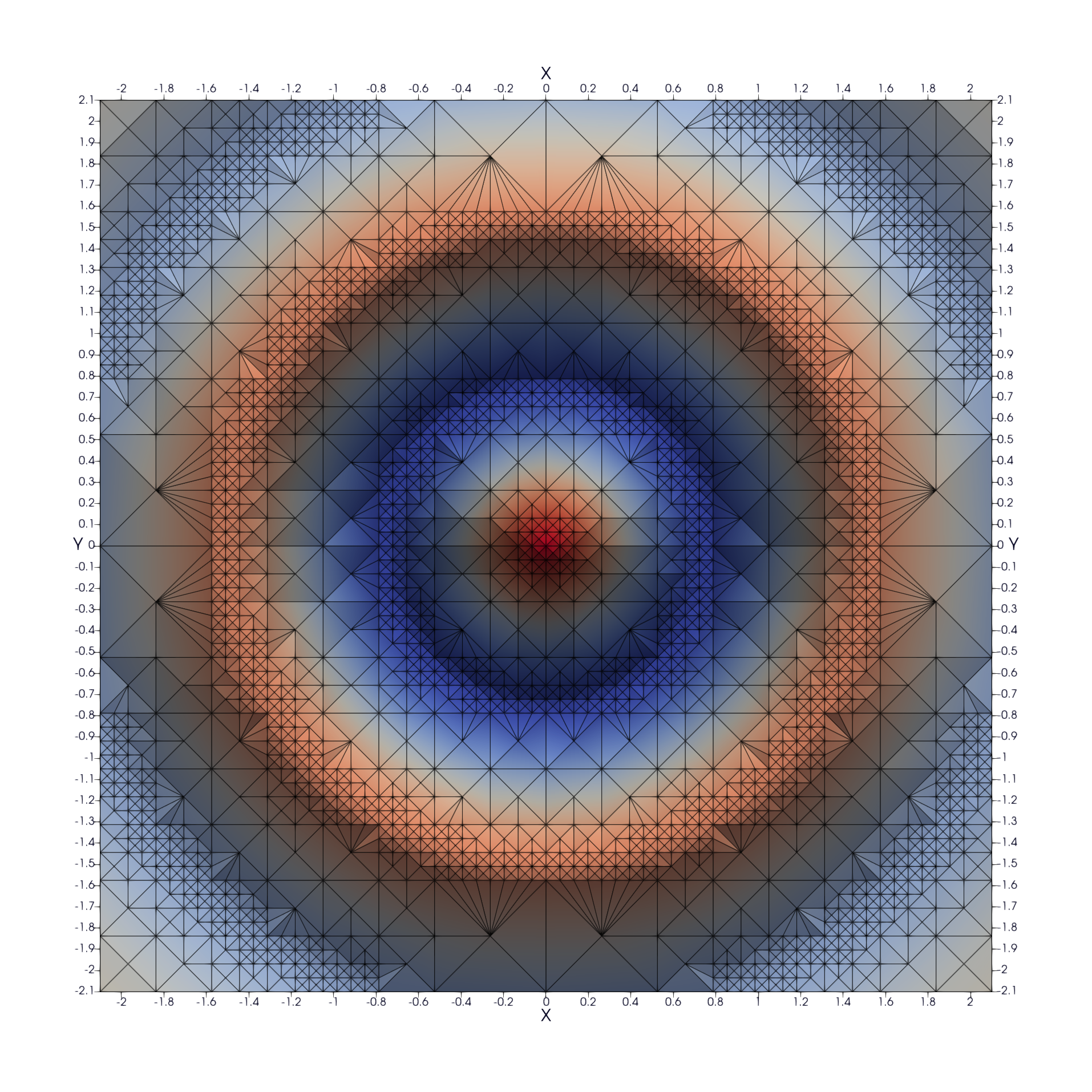
One popular way to plot complex functions is to use a surface plot of $| f (z) |$ and color the surface with $\arg (f (z))$ . This way we can simultaneously represent the magnitude and phase over the complex plain. There are several ways to color the plots, and we will be following the method described by Richardson in 1991. In this example, we demonstrates several techniques:

Alternate ways to do an initial sample (grid vs recursive)
Sample near a point in the domain
Sample below a level in the range
Sample near level curves
Sample based on a data value that is not part of the geometry
Sample near domain axis
Use MRaster to compute colors for complex numbers
Directly attach colors to geometric points
Do rough clipping with high sampling and cell filtering.
Precision clipping by folding & culling.

Paraview State File: https://github.com/richmit/MRPTree/blob/main/paraview/complex_magnitude_surface.pvsm

XML VTK Data File: https://github.com/richmit/MRPTree/blob/main/paraview/complex_magnitude_surface.vtu

Source code: https://github.com/richmit/MRPTree/blob/main/examples/complex_magnitude_surface.cpp

#include "MR_rect_tree.hpp"
#include "MR_cell_cplx.hpp"
#include "MR_rt_to_cc.hpp"
#include "MRcolor.hpp"

typedef mjr::tree15b2d9rT            tt_t;
typedef mjr::MRccT5                  cc_t;
typedef mjr::MR_rt_to_cc<tt_t, cc_t> tc_t;
typedef mjr::color3c64F              ct_t;

tt_t::rrpt_t cpf(tt_t::drpt_t xvec) {
  std::complex<double> z(xvec[0], xvec[1]);
  double z_abs, z_arg, f_re, f_im, f_abs, f_arg, red, green, blue;

  z_abs = std::abs(z);
  z_arg = std::arg(z);

  if ( (std::abs(z-1.0) > 1.0e-5) && (std::abs(z+1.0) > 1.0e-5) ) {
    std::complex<double> f;
    f        = 1.0/(z+1.0) + 1.0/(z-1.0);
    f_re     = std::real(f);
    f_im     = std::imag(f);
    f_abs    = std::abs(f);
    f_arg    = std::arg(f);
    ct_t c   = ct_t::cs2dIdxPalArg<ct_t::csCColdeRainbow, 3, 5.0, 20.0, 2.0, 1>::c(f); 
    red      = c.getRed();
    green    = c.getGreen();
    blue     = c.getBlue();
  } else {
    f_re = f_im = f_abs = f_arg = red = green = blue = std::numeric_limits<double>::quiet_NaN();
  }

  return {z_abs, z_arg, f_re, f_im, f_abs, f_arg, red, green, blue};
}

tt_t::src_t  cpfd(tt_t::drpt_t xvec) {
  int    idx_for_z = 4;
  double cut_for_z = 3.5;
  auto   fv        = cpf(xvec);

  if(std::isnan(fv[idx_for_z]))
    return 100000.0;
  else
    return fv[idx_for_z]-cut_for_z;
}

int main() {
  tt_t tree({-2.2, -1.2}, 
            { 2.2,  1.2});
  cc_t ccplx;

  // Initial sample

  // On a uniform grid
  tree.refine_grid(7, cpf);

  // Alternately we can use refine_recursive() instead (refine_grid() is faster)
  // tree.refine_recursive(4, cpf);

  // Sample near 0+0i because we have a minimum at that piont

  // The most direct method 
  // tree.refine_leaves_recursive_cell_pred(6, cpf, [&tree](tt_t::diti_t i) { return (tree.cell_close_to_domain_point({0, 0}, 1.0e-2, i)); });

  // This function is positive with a universal minimum at 0+0i, so we could just sample where  |f| is below 1/4
  tree.refine_leaves_recursive_cell_pred(6, cpf, [&tree](tt_t::diti_t i) { return !(tree.cell_above_range_level(i, 4, 0.25, 1.0e-5)); });

  // Sample around the poles where we will clip the graph

  // With nice ranges the singularities will be precicely located on cell vertexes.  So we can just refine NaNs.
  // tree.refine_recursive_if_cell_vertex_is_nan(6, cpf);

  // Or we can directly sample on the clip level at |f|=3.5.  
  tree.refine_leaves_recursive_cell_pred(7, cpf, [&tree](tt_t::diti_t i) { return (tree.cell_cross_range_level(i, 4, 3.5)); });

  // We can do the above with a constructed SDF instead.
  // tree.refine_leaves_recursive_cell_pred(6, cpf, [&tree](tt_t::diti_t i) { return (tree.cell_cross_sdf(i, cpfd)); });

  // Just like the previous, but with atomic refinement.
  // tree.refine_leaves_atomically_if_cell_pred(6, cpf, [&tree](tt_t::diti_t i) { return (tree.cell_cross_sdf(i, cpfd)); });

  // Refine where we plan to draw level curves

  // The easiest thing is to use cell_cross_range_level() for this.
  for(auto lev: {0.4, 0.7, 1.1, 1.4, 1.8, 2.6, 3.5}) 
    tree.refine_leaves_recursive_cell_pred(7, cpf, [&tree, lev](tt_t::diti_t i) { return (tree.cell_cross_range_level(i, 4, lev)); });

  // We will be coloring based on arg(f), and so want to sample near the abrubpt change near arg(f)=0.

  // We can do this just like the level curves with |f|, but use arg(f) instead -- i.e. index 5 instead of 4.
  tree.refine_leaves_recursive_cell_pred(7, cpf, [&tree](tt_t::diti_t i) { return (tree.cell_cross_range_level(i, 5, 0.0)); });

  // We can sample near the real & imagaxes axes.

  // Sample near the real axis
  tree.refine_leaves_recursive_cell_pred(5, cpf, [&tree](tt_t::diti_t i) { return (tree.cell_cross_domain_level(i, 0, 0.0, 1.0e-6)); });

  // Sample near the imaginary axis
  tree.refine_leaves_recursive_cell_pred(5, cpf, [&tree](tt_t::diti_t i) { return (tree.cell_cross_domain_level(i, 1, 0.0, 1.0e-6)); });

  // We don't need to balance the three, but it makes things look nice.

  // Balance the three to the traditional level of 1 (no  cell borders a cell more than half it's size)
  tree.balance_tree(1, cpf);

  // At this point the tree is adequately sampled, so we print a bit out to the screen.
  tree.dump_tree(5);

  // Create the cell complex from cells that have at least one point below our clipping plane.
  auto tcret = tc_t::construct_geometry_fans(ccplx,
                                             tree,
                                             tree.get_leaf_cells_pred(tree.ccc_get_top_cell(), 
                                                                      [&tree](tt_t::diti_t i) { return !(tree.cell_above_range_level(i, 4, 3.5, 1.0e-6)); }),
                                             2,
                                             {{tc_t::val_src_spc_t::FDOMAIN, 0}, 
                                              {tc_t::val_src_spc_t::FDOMAIN, 1},
                                              {tc_t::val_src_spc_t::FRANGE,  4}});
  std::cout << "TC Return: " << tcret << std::endl;
  ccplx.create_named_datasets({"Re(z)", "Im(z)", "abs(z)", "arg(z)", "Re(f(z))", "Im(f(z))", "abs(f(z))", "arg(f(z))"}, {{"COLORS", {8, 9, 10}}});
  std::cout << "POST CONST" << std::endl;
  ccplx.dump_cplx(5);

  // Fold the triangles on our clipping plane
  ccplx.triangle_folder([](cc_t::node_data_t x){return tc_t::tsampf_to_cdatf(        cpf, x); }, 
                        [](cc_t::node_data_t x){return tc_t::tsampf_to_clcdf(4, 3.5, cpf, x); });
  std::cout << "POST FOLD" << std::endl;
  ccplx.dump_cplx(5);

  // Remove all triangles above our clipping plane

  // We can do this directly with ccplx using index 6 into the point data (point data is domain data appended with range data)
  // ccplx.cull_cells([&ccplx](cc_t::cell_verts_t c){ return !(ccplx.cell_below_level(c, 6, 3.5)); });

  // Or we can use the index in the original sample function along with the converter rt_rng_idx_to_pd_idx().
  ccplx.cull_cells([&ccplx](cc_t::cell_verts_t c){ return !(ccplx.cell_below_level(c, tc_t::rt_rng_idx_to_pd_idx(4), 3.5)); });

  std::cout << "POST CULL" << std::endl;
  ccplx.dump_cplx(5);

  ccplx.write_legacy_vtk("complex_magnitude_surface.vtk", "complex_magnitude_surface");
  ccplx.write_xml_vtk(   "complex_magnitude_surface.vtu", "complex_magnitude_surface");
  ccplx.write_ply(       "complex_magnitude_surface.ply", "complex_magnitude_surface");
}

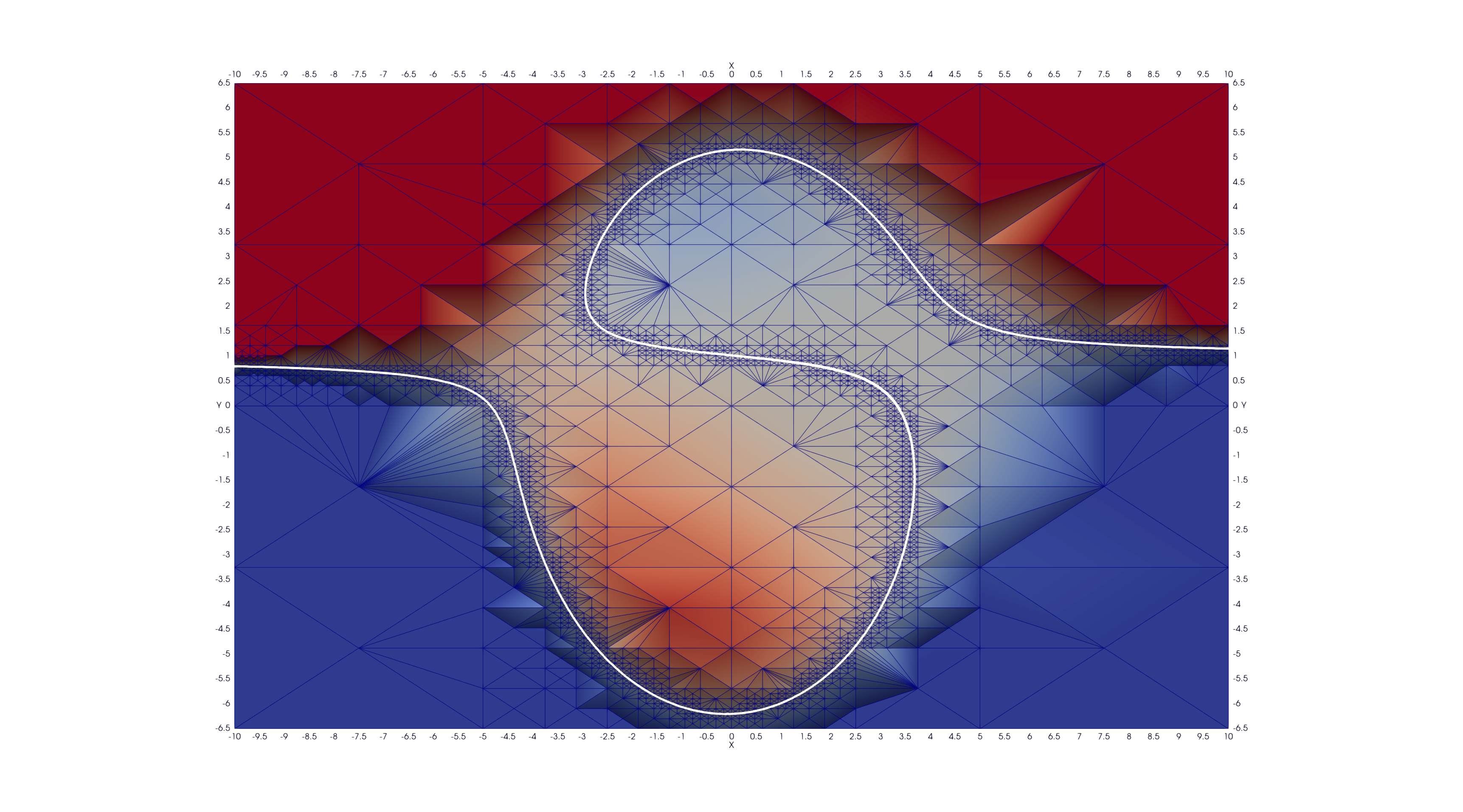
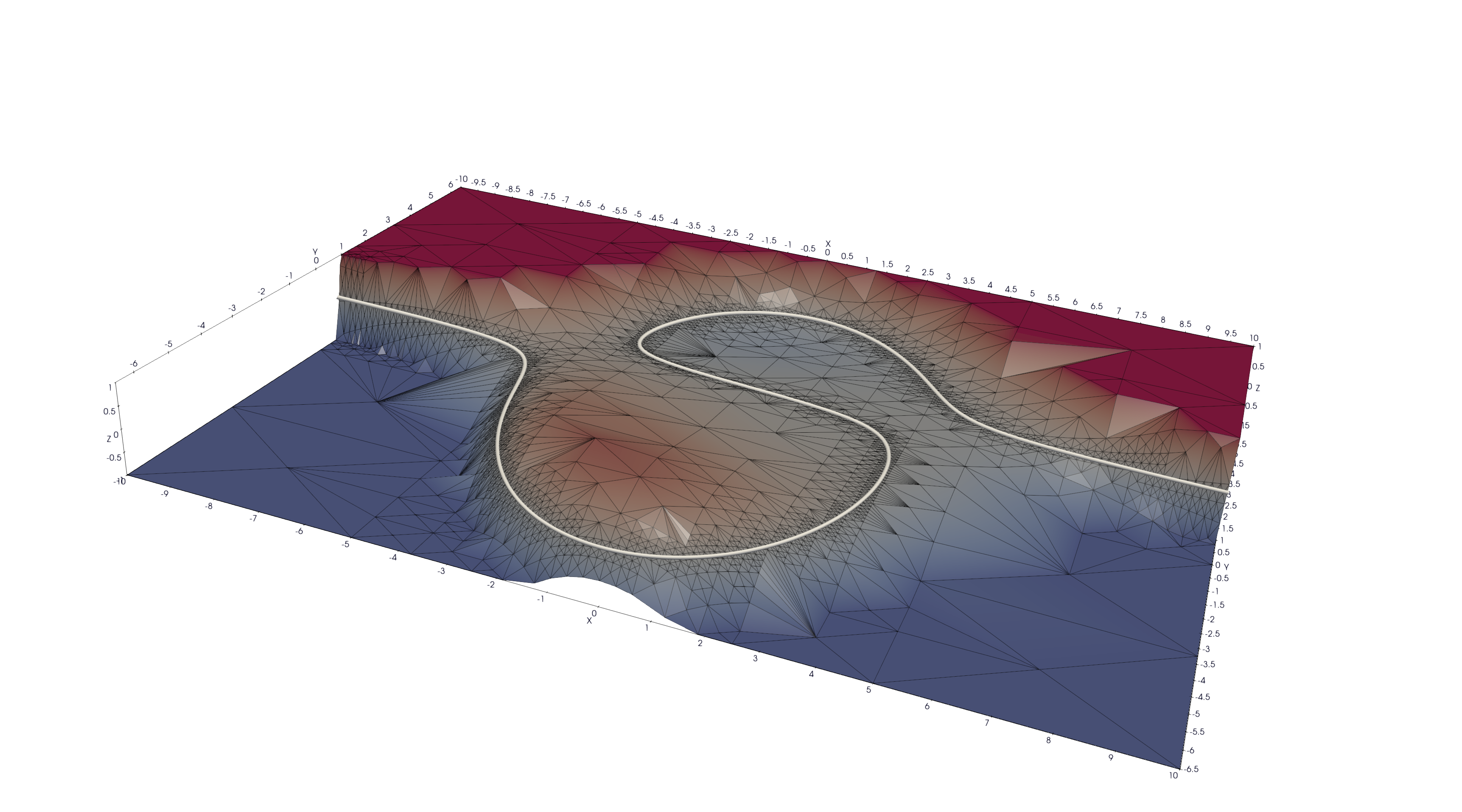
2.2. Implicit Curve

For many of us our first exposure to an implicit curve was the unit circle in high school algebra, $x^{2} + y^{2} = 1$ , where we were ask to graph $y$ with respect to $x$ only to discover that $y$ didn't appear to be a function of $x$ because $y$ had TWO values for some values of $x$ ! But we soon discovered that a great many interesting curves could be defined this way, and that we could represent them all by thinking of the equations as a functions of two variables and the curves as sets of zeros. That is to say, we can always write an implicit equation in two variables in the form $F (x, y) = 0$ , and think of the implicit curve as the set of roots, or zeros, of the function $F$ . We can then generalize this idea to "level sets" as solutions to $F (x, y) = L$ – i.e. the set of points where the function is equal to some "level" $L$ .

Many visualization tools can extract a "level set" from a mesh. For 2D meshes (surfaces), the level sets are frequently 1D sets (curves). The trick to obtaining high quality results is to make sure the triangulation has a high enough resolution. Of course we could simply sample the 2D grid uniformly with a very fine mesh. A better way is to detect where the curve is, and to sample at higher resolution near the curve.

Currently we demonstrate a couple ways to refine the mesh near the curve:

Using cell_cross_range_level() to find cells that cross a particular level (zero in this case)
Using cell_cross_sdf() instead – which generally works just like cell_cross_range_level() with a level of zero.

Today we extract the curve with Paraview, but I hope to extend MR_rt_to_cc to extract level sets in the future:

Extract "standard" midpoint level sets (TBD)
Solve for accurate edge/function level intersections, and construct high quality level sets. (TBD)

Paraview State File: https://github.com/richmit/MRPTree/blob/main/paraview/implicit_curve_2d.pvsm

XML VTK Data File: https://github.com/richmit/MRPTree/blob/main/paraview/implicit_curve_2d.vtu

Source code: https://github.com/richmit/MRPTree/blob/main/examples/implicit_curve_2d.cpp

#include "MR_rect_tree.hpp"
#include "MR_cell_cplx.hpp"
#include "MR_rt_to_cc.hpp"

typedef mjr::tree15b2d1rT            tt_t;
typedef mjr::MRccT5                  cc_t;
typedef mjr::MR_rt_to_cc<tt_t, cc_t> tc_t;

// This function is a classic "difficult case" for implicit curve algorithms.
tt_t::rrpt_t f(tt_t::drpt_t xvec) {
  double x = xvec[0];
  double y = xvec[1];
  double z = ((2*x*x*y - 2*x*x - 3*x + y*y*y - 33*y + 32) * ((x-2)*(x-2) + y*y + 3))/3000;
  if (z>1.0)
    z=1.0;
  if (z<-1.0)
    z=-1.0;
  return z;
}

int main() {
  tt_t tree({-10.0, -6.5},
            { 10.0,  6.5});
  cc_t ccplx;

  // First we sample the top cell.  Just one cell!
  tree.sample_cell(f);

  // Now we recursively refine cells that seem to cross over the curve
  tree.refine_leaves_recursive_cell_pred(7, f, [&tree](tt_t::diti_t i) { return (tree.cell_cross_range_level(i, 0, 0.0)); });

  // We could have used the function f as an SDF, and achieved the same result with the following:
  // tree.refine_leaves_recursive_cell_pred(7, f, [&tree](tt_t::diti_t i) { return (tree.cell_cross_sdf(i, f)); });

  tree.dump_tree(20);

  // Convert the geometry into a 3D dataset so we can see the contour on the surface
  tc_t::construct_geometry_fans(ccplx,
                                tree,
                                2,
                                {{tc_t::val_src_spc_t::FDOMAIN, 0},
                                 {tc_t::val_src_spc_t::FDOMAIN, 1},
                                 {tc_t::val_src_spc_t::FRANGE,  0}});

  ccplx.create_named_datasets({"x", "y", "f(x,y)"});

  ccplx.write_xml_vtk("implicit_curve_2d.vtu", "implicit_curve_2d");
}

2.3. Implicit Surface

This example is very similar to implicit_curve_2d.cpp; however, instead of extracting a curve from a triangulation of a surface, this time we extract a surface from a quad tessellation of a hexahedron. In addition to what we demonstrate with implicit_curve_2d.cpp, this example also demonstrates:

How to use an SDF to identify cells that contain the level set
How to export only a subset of cells

Paraview State File: https://github.com/richmit/MRPTree/blob/main/paraview/implicit_surface.pvsm

XML VTK Data File: https://github.com/richmit/MRPTree/blob/main/paraview/implicit_surface.vtu

Source code: https://github.com/richmit/MRPTree/blob/main/examples/implicit_surface.cpp

#include "MR_rect_tree.hpp"
#include "MR_cell_cplx.hpp"
#include "MR_rt_to_cc.hpp"

typedef mjr::tree15b3d1rT            tt_t;
typedef mjr::MRccT5                  cc_t;
typedef mjr::MR_rt_to_cc<tt_t, cc_t> tc_t;

tt_t::rrpt_t isf(tt_t::drpt_t xvec) {
  double x = xvec[0];
  double y = xvec[1];
  double z = xvec[2];
  return x*x*y+y*y*x-z*z*z-1;
}

int main() {
  tt_t tree({-2.3, -2.3, -2.3}, 
            { 2.3,  2.3,  2.3});
  cc_t ccplx;

  /* Initial uniform sample */
  tree.refine_grid(4, isf);

  /* Refine near surface */
  tree.refine_leaves_recursive_cell_pred(6, isf, [&tree](tt_t::diti_t i) { return (tree.cell_cross_sdf(i, isf)); });

  tree.dump_tree(5);

  /* Convert our tree to a cell complex.  Note that we use an SDF to export only cells that contain our surface */
  tc_t::construct_geometry_rects(ccplx,
                                 tree,
                                 tree.get_leaf_cells_pred(tree.ccc_get_top_cell(), [&tree](tt_t::diti_t i) { return (tree.cell_cross_sdf(i, isf)); }),
                                 3,
                                 {{tc_t::val_src_spc_t::FDOMAIN, 0}, 
                                  {tc_t::val_src_spc_t::FDOMAIN, 1},
                                  {tc_t::val_src_spc_t::FDOMAIN, 2}});

  /* Name the data points */
  ccplx.create_named_datasets({"x", "y", "z", "f(x,y,z)"});

  /* Display some data about the cell complex */
  ccplx.dump_cplx(5);

  /* Write out our cell complex */
  ccplx.write_xml_vtk("implicit_surface.vtu", "implicit_surface");
}

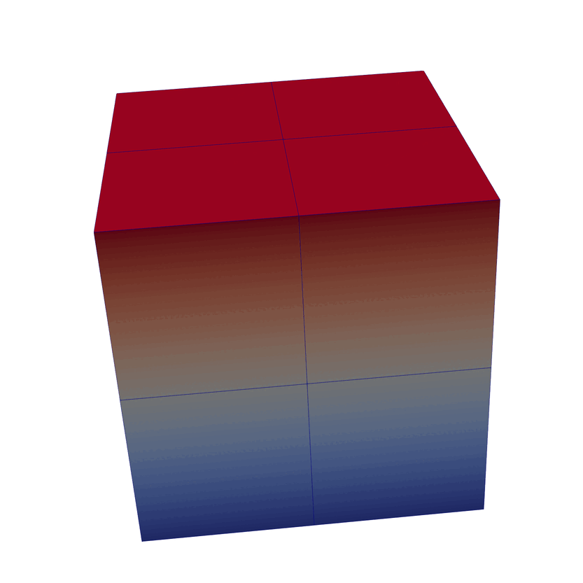
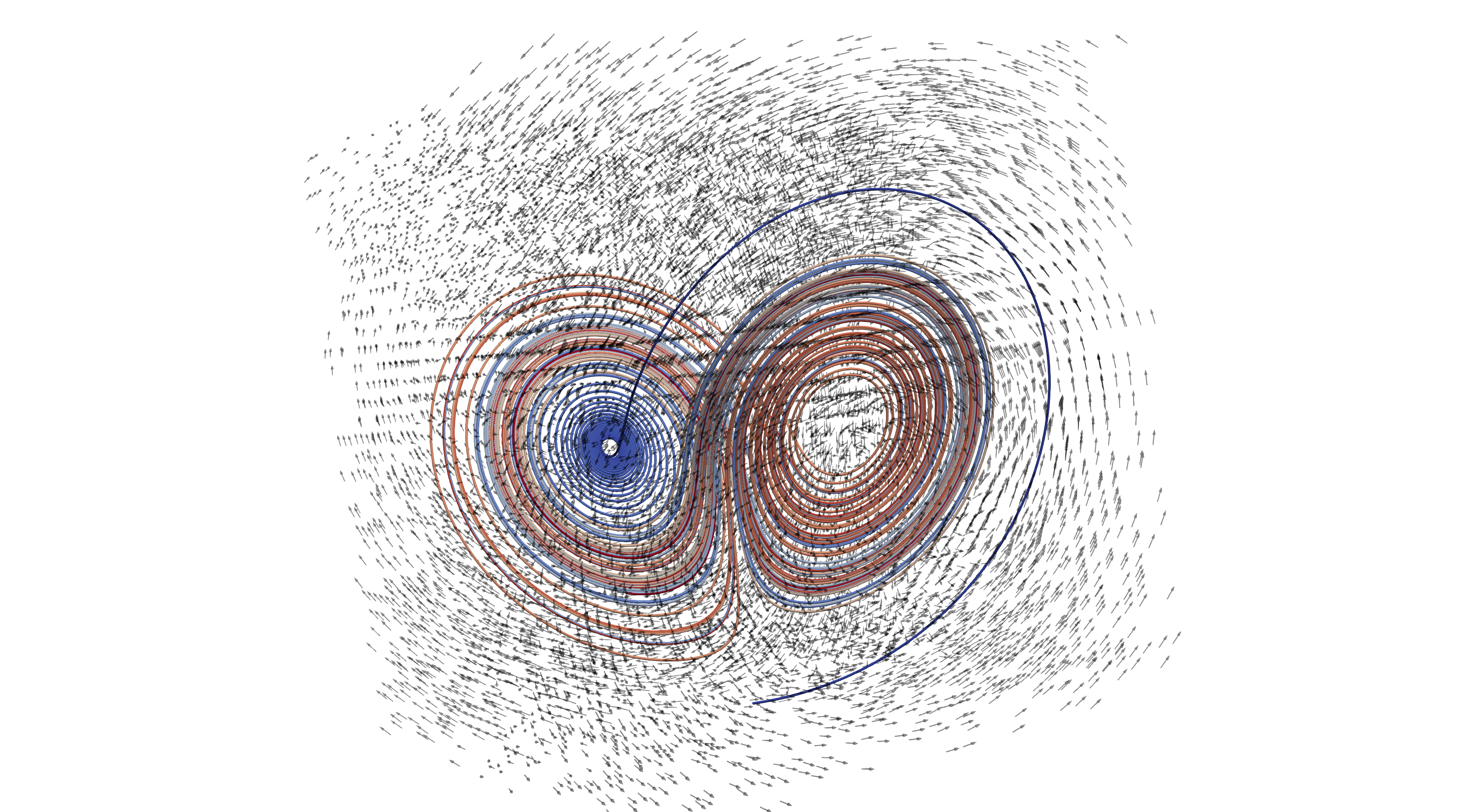
2.4. 3D Vector Field

This example illustrates how to uniformly sample a vector field. Just for fun we have also produced a solution to the Lorenz system, and directly stored it with a MR_cell_cplx.

XML VTK Data File 1: https://github.com/richmit/MRPTree/blob/main/paraview/vector_field_3d-c.vtu

XML VTK Data File 2: https://github.com/richmit/MRPTree/blob/main/paraview/vector_field_3d-f.vtu

Source code: https://github.com/richmit/MRPTree/blob/main/examples/vector_field_3d.cpp

#include "MR_rect_tree.hpp"
#include "MR_cell_cplx.hpp"
#include "MR_rt_to_cc.hpp"

typedef mjr::tree15b3d3rT            tt_t;
typedef mjr::MRccT5                  cc_t;
typedef mjr::MR_rt_to_cc<tt_t, cc_t> tc_t;

tt_t::rrpt_t vf(tt_t::drpt_t xvec) {
  double x = xvec[0];
  double y = xvec[1];
  double z = xvec[2];
  double a = 10.0;
  double b = 28.0;
  double c = 8.0/3.0;
  return { a*y-a*z,
           x*b-x*z,
           x*y-c*z
         };
}                          

int main() {
  tt_t vftree({-30.0, -30.0,  -0.0},
              { 30.0,  30.0,  60.0});
  cc_t vfccplx;

  /* Uniform sampling */
  vftree.refine_grid(5, vf);

  /* Dump the vector field */
  tc_t::construct_geometry_rects(vfccplx,
                                 vftree,
                                 0,
                                 {{tc_t::val_src_spc_t::FDOMAIN,  0},
                                  {tc_t::val_src_spc_t::FDOMAIN,  1},
                                  {tc_t::val_src_spc_t::FDOMAIN,  2}});

  vfccplx.create_named_datasets({"x", "y", "z"},
                                {{"d", {0, 1, 2}}});
  vfccplx.dump_cplx(5);
  vfccplx.write_xml_vtk("vector_field_3d-f.vtu", "vector_field_3d-f");

  /* Now we solve the Lorenz system and directly create a cc_t object */
  cc_t cvccplx;

  int max_steps = 100000;
  double delta  = 0.001;
  double t      = 0;
  double x_old  = 0.1;
  double y_old  = 0.0;
  double z_old  = 0.0;
  double a      = 10.0;
  double b      = 28.0;
  double c      = 8.0 / 3.0;

  auto p_old = cvccplx.add_node({x_old, y_old, z_old, t});
  for(int num_steps=0;num_steps<max_steps;num_steps++) {    
    double x_new = x_old + a*(y_old-x_old)*delta;
    double y_new = y_old + (x_old*(b-z_old)-y_old)*delta;
    double z_new = z_old + (x_old*y_old-c*z_old)*delta;
    t += delta;
    auto p_new = cvccplx.add_node({x_new, y_new, z_new, t});
    cvccplx.add_cell(cc_t::cell_kind_t::SEGMENT, {p_old, p_new});
    x_old=x_new;
    y_old=y_new;
    z_old=z_new;
    p_old=p_new;
  }

  cvccplx.dump_cplx(5);
  cvccplx.write_xml_vtk("vector_field_3d-c.vtu", "vector_field_3d-c");
}

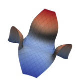
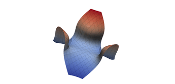
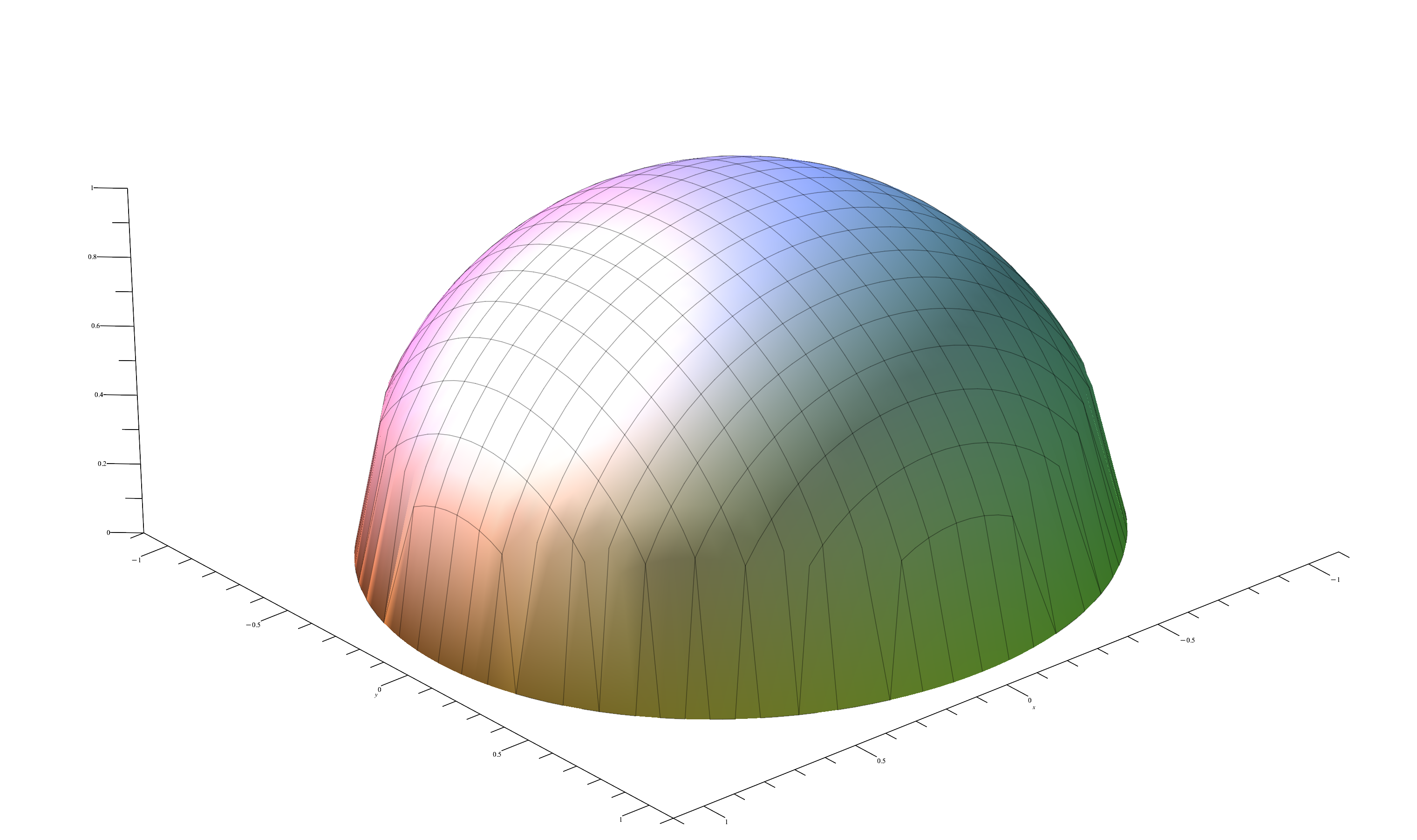
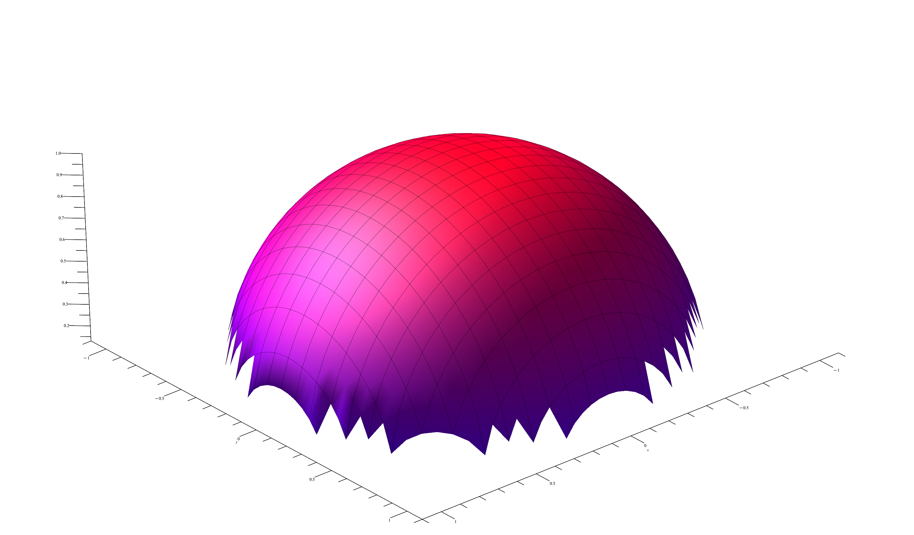
2.5. Surface Plot With Normals

Surface normals may be used by many visualization tools to render smoother results. In this example we demonstrate:

How to compute a surface gradient for a function plot
How to unitize the gradient into a surface normal
How to add the normal to the sample data stored by a MRPTree
How to include normals in the cell complex
How to increase sampling with a SDF function
How to increase sampling near humps by testing derivatives
How to balance a tree
How to dump a cell complex into various file types

Surfaces with and without normals

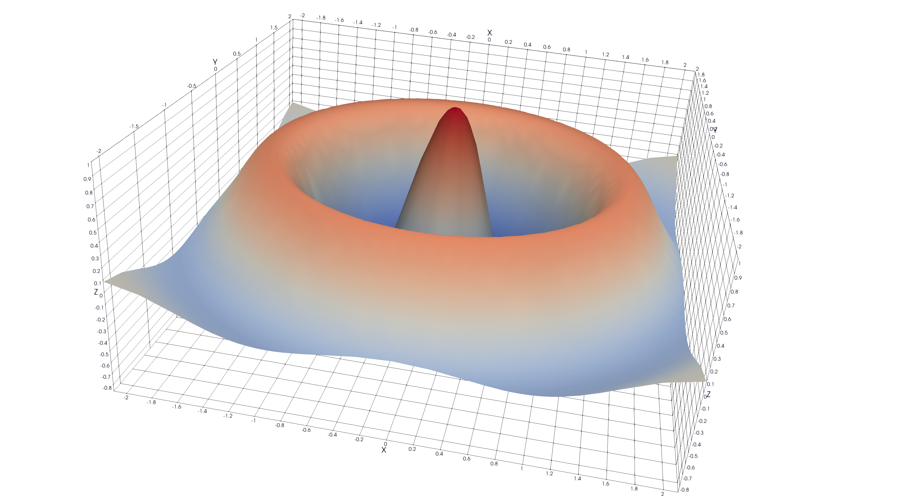
The mesh without any refinement

The mesh with refinement (sdf, partial derivative, directional derivative)

Mesh with directional directional refinement but unbalanced)

Paraview State File: https://github.com/richmit/MRPTree/blob/main/paraview/surface_with_normals.pvsm

XML VTK Data File: https://github.com/richmit/MRPTree/blob/main/paraview/surface_with_normals.vtu

Source code: https://github.com/richmit/MRPTree/blob/main/examples/surface_with_normals.cpp

#include "MR_rect_tree.hpp"
#include "MR_cell_cplx.hpp"
#include "MR_rt_to_cc.hpp"

typedef mjr::tree15b2d5rT            tt_t;
typedef mjr::MRccT5                  cc_t;
typedef mjr::MR_rt_to_cc<tt_t, cc_t> tc_t;

tt_t::rrpt_t damp_cos_wave(tt_t::drpt_t xvec) {
  double x = xvec[0];
  double y = xvec[1];
  double d = x*x+y*y;
  double m = std::exp(-d/4);
  double s = std::sqrt(d);
  double z = m*cos(4*s);
  double dx = -(cos((4 * s)) * s + 4 * sin( (4 * s))) * x * exp(-x * x / 2 - y * y / 2);
  double dy = -(cos((4 * s)) * s + 4 * sin( (4 * s))) * y * exp(-x * x / 2 - y * y / 2);
  double dd =   -m*(cos(4*s)*s+8*sin(4*s));
  if (s>1.0e-5) {
    dx = dx / s;
    dy = dy / s;
    dd = dd / (4 * s);
  } else {
    dx = 1;
    dy = 1;
    dd = 1;
  }
  double nm = std::sqrt(1+dx*dx+dy*dy);
  return {z, -dx/nm, -dy/nm, 1/nm, dd};
}

double circle_sdf(double r, tt_t::drpt_t xvec) {
  double x = xvec[0];
  double y = xvec[1];
  double m = x*x+y*y;
  return (r*r-m);
}

int main() {
  tt_t tree({-2.1, -2.1}, 
            { 2.1,  2.1});
  cc_t ccplx;

  // Make a few samples on a uniform grid
  tree.refine_grid(2, damp_cos_wave);

  // The humps need extra samples.  We know where they are, and we could sample on them with an SDF like this:
  // for(double i: {0, 1, 2, 3}) {
  //   double r = i*std::numbers::pi/4;
  //   tree.refine_leaves_recursive_cell_pred(6, damp_cos_wave, [&tree, r](int i) { return (tree.cell_cross_sdf(i, std::bind_front(circle_sdf, r))); });
  // }

  // Alternately, we can test the derivative values to identify the humps
  // tree.refine_leaves_recursive_cell_pred(6, damp_cos_wave, [&tree](tt_t::diti_t i) { return tree.cell_cross_range_level(i, 1, 0.0); });
  // tree.refine_leaves_recursive_cell_pred(6, damp_cos_wave, [&tree](tt_t::diti_t i) { return tree.cell_cross_range_level(i, 2, 0.0); });

  // Lastly we can use the directional derivative radiating from the origin
  tree.refine_leaves_recursive_cell_pred(6, damp_cos_wave, [&tree](tt_t::diti_t i) { return tree.cell_cross_range_level(i, 4, 0.0); });

  // Balance the three to the traditional level of 1 (no  cell borders a cell more than half it's size)
  tree.balance_tree(1, damp_cos_wave);

  tree.dump_tree(5);

  tc_t::construct_geometry_fans(ccplx,
                                tree,
                                2,
                                {{tc_t::val_src_spc_t::FDOMAIN, 0}, 
                                 {tc_t::val_src_spc_t::FDOMAIN, 1},
                                 {tc_t::val_src_spc_t::FRANGE,  0}});

  // Note we use the single argument version of create_named_datasets() because we don't want to name elements 3, 4, & 5 (the components of the normal
  // Note if we had placed the ddiv component right after z, then we could have used the two argument version...
  ccplx.set_data_name_to_data_idx_lst({{"x",        {0}},
                                       {"y",        {1}},
                                       {"z=f(x,y)", {2}},
                                       {"ddiv",     {6}},
                                       {"NORMALS",  {3,4,5}}});

  ccplx.dump_cplx(5);

  ccplx.write_legacy_vtk("surface_with_normals.vtk", "surface_with_normals");
  ccplx.write_xml_vtk(   "surface_with_normals.vtu", "surface_with_normals");
  ccplx.write_ply(       "surface_with_normals.ply", "surface_with_normals");
}

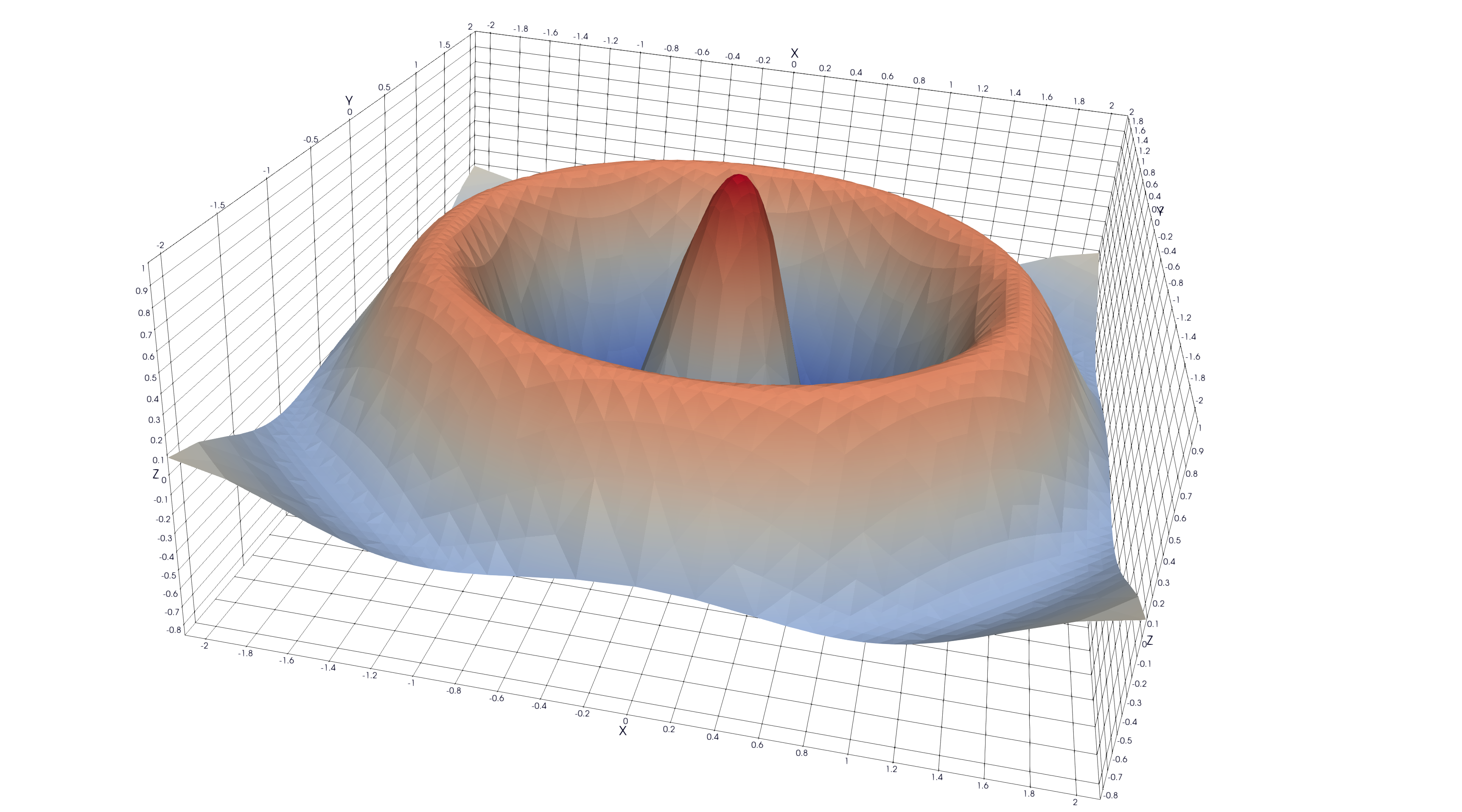
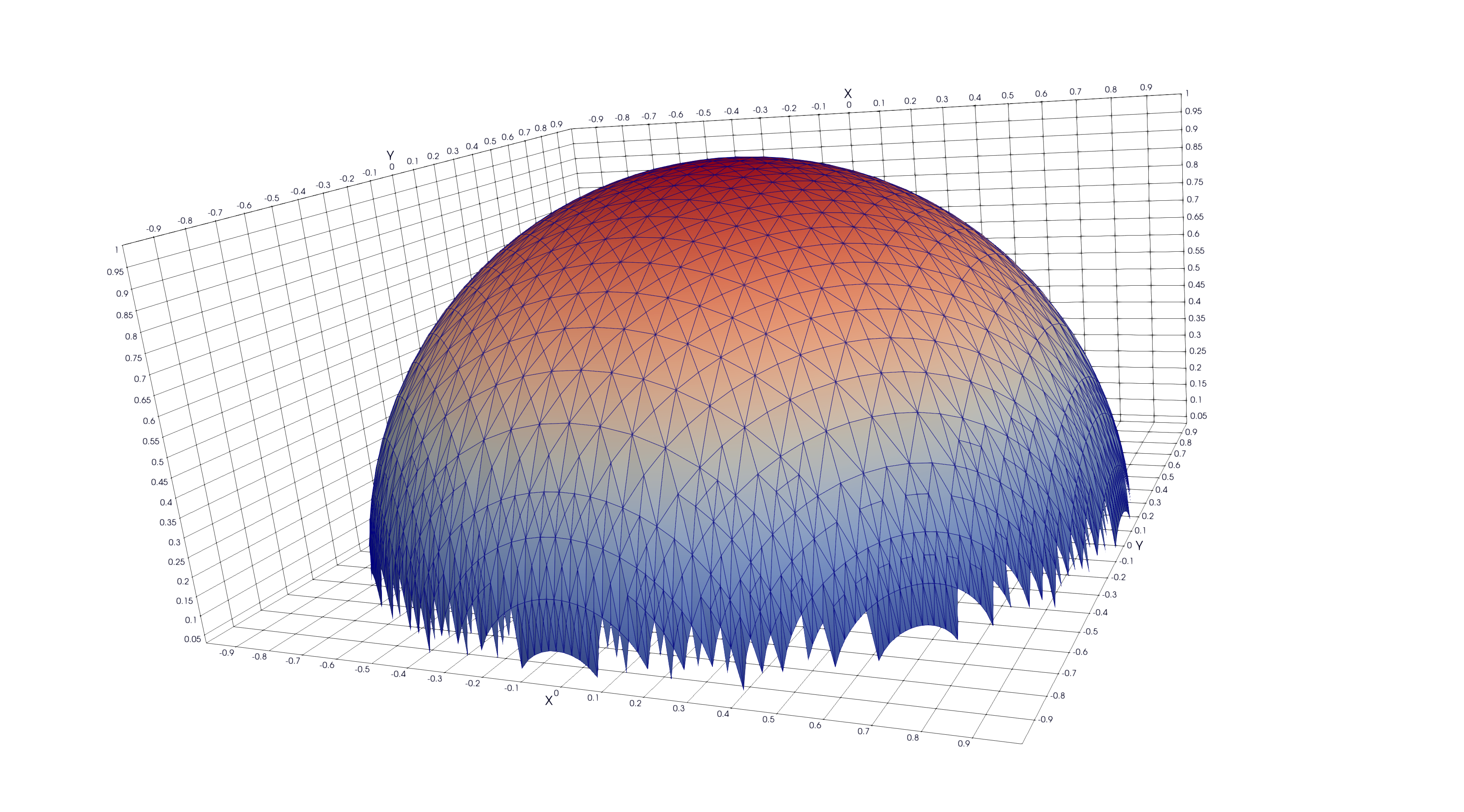
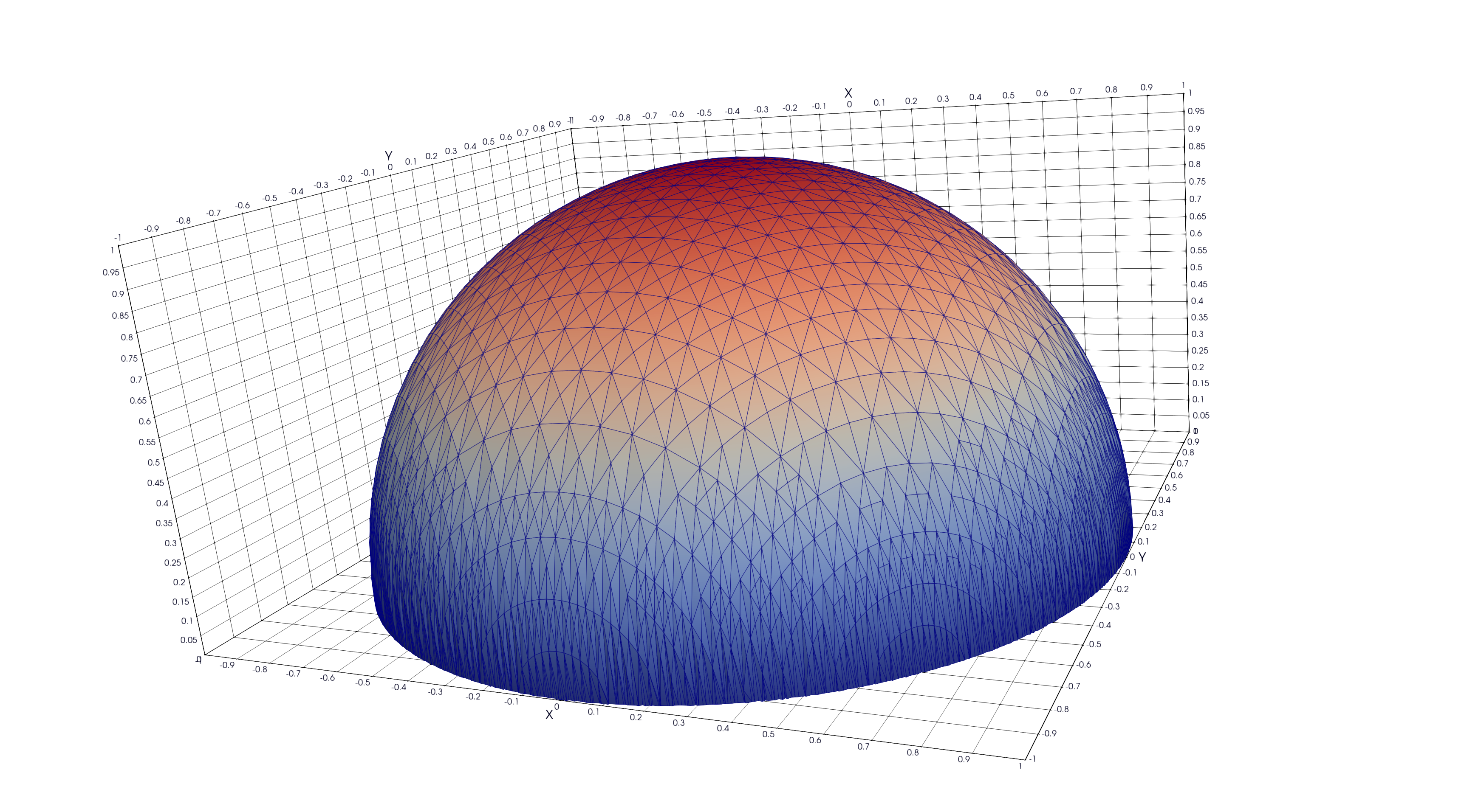
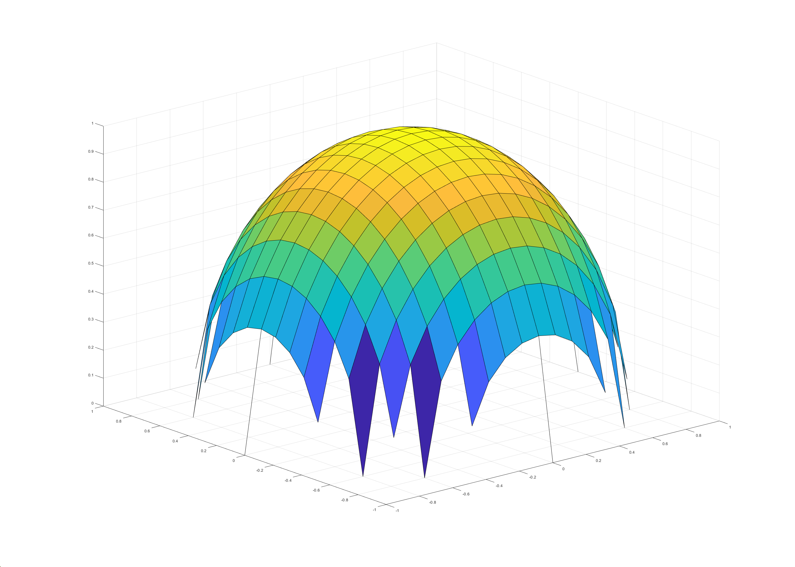
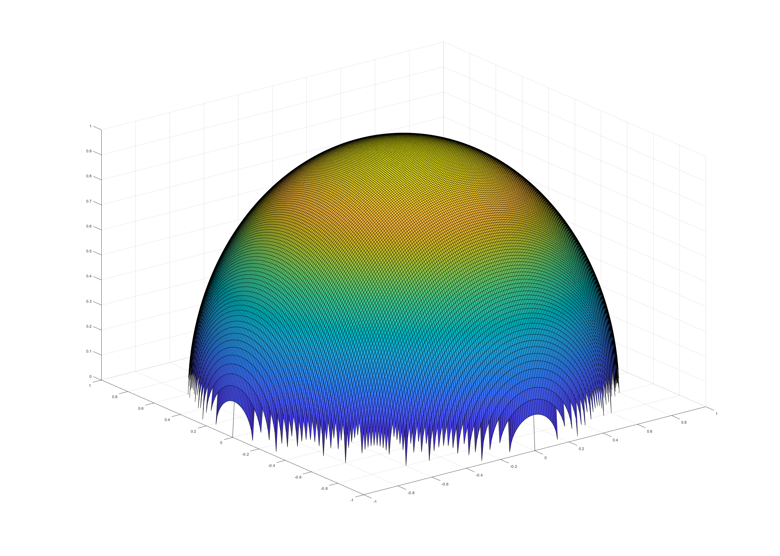
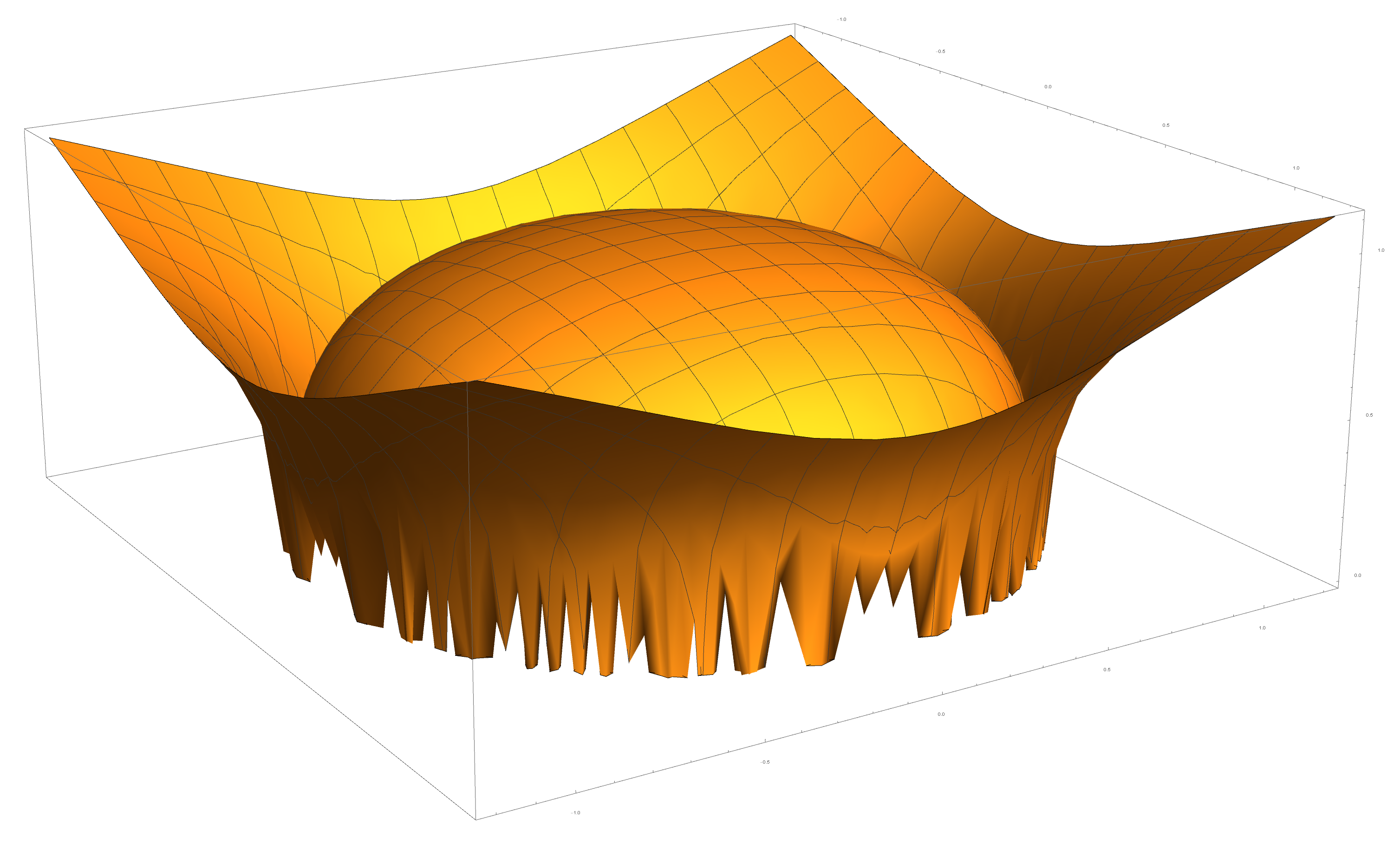
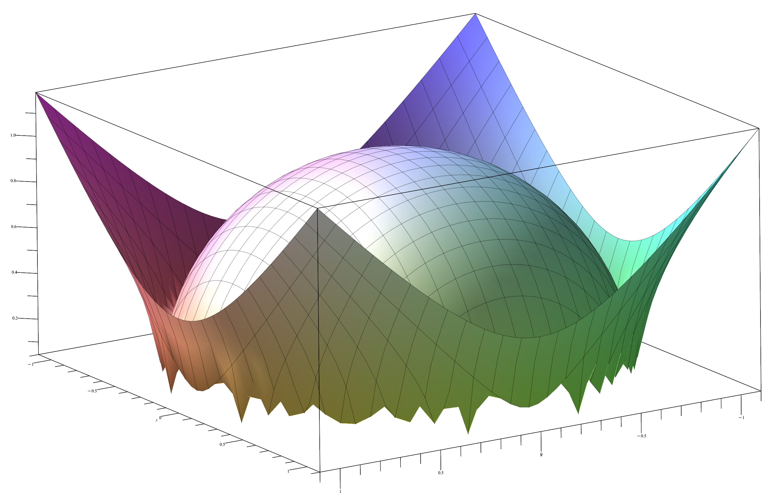
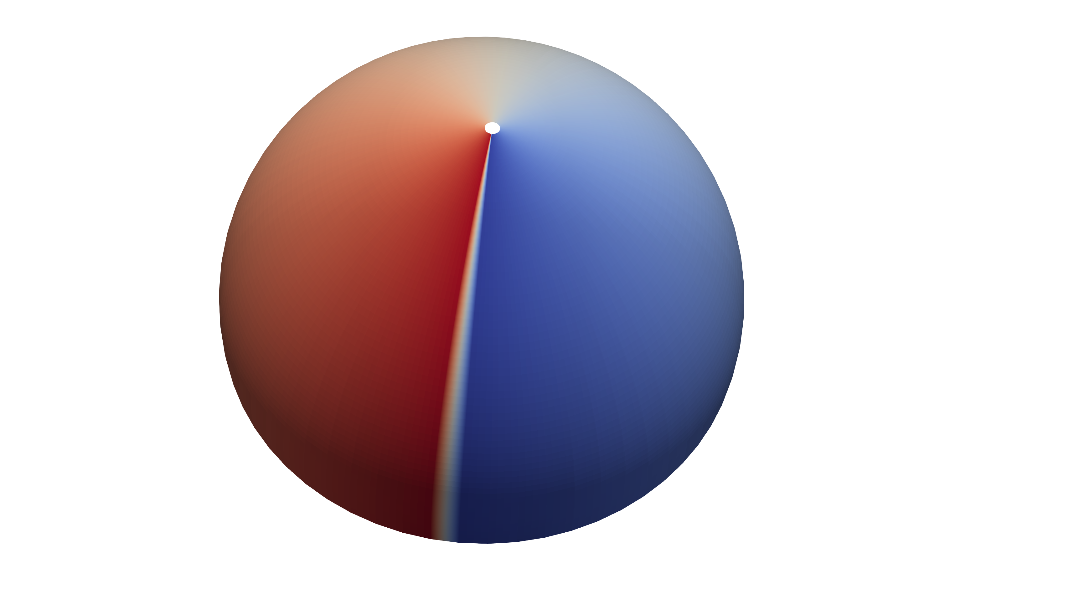
2.6. Surface Plot With An Edge

Surface plots are frequently complicated by regions upon which the function singular or undefined. These functions often behave quite poorly on the boundaries of such regions. For this example we consider $f (x, y) = \sqrt{1 - x^{2} - y^{2}}$ – the upper half of the unit sphere. Outside the unit circle this function is complex. As we approach the unit circle from the center, the derivative approaches infinity.

Right now this example illustrates two things:

How to drive up the sample rate near NaNs.
How to repair triangles containing NaNs.

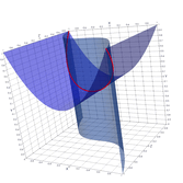
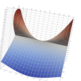
Typical Jagged Edge vs Healed Edge

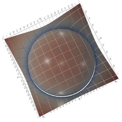
Examples From Matlab (Coarse & Fine Mesh)

Examples From Maple (With & Without Adaptive Mesh)

Paraview State File: https://github.com/richmit/MRPTree/blob/main/paraview/surface_plot_edge.pvsm

XML VTK Data File: https://github.com/richmit/MRPTree/blob/main/paraview/surface_plot_edge.vtu

Source code: https://github.com/richmit/MRPTree/blob/main/examples/surface_plot_edge.cpp

#include "MR_rect_tree.hpp"
#include "MR_cell_cplx.hpp"
#include "MR_rt_to_cc.hpp"

typedef mjr::tree15b2d1rT            tt_t;
typedef mjr::MRccT5                  cc_t;
typedef mjr::MR_rt_to_cc<tt_t, cc_t> tc_t;

tt_t::rrpt_t half_sphere(tt_t::drpt_t xvec) {
  double m = xvec[0] * xvec[0] + xvec[1] * xvec[1];
  if (m > 1) {
    return std::numeric_limits<double>::quiet_NaN();
  } else {
    return std::sqrt(1-m);
  }
}

int main() {
  tt_t tree({-1.1, -1.1}, 
            { 1.1,  1.1});
  cc_t ccplx;

  // Sample a uniform grid across the domain
  tree.refine_grid(5, half_sphere);

  /* half_sphere produces NaNs outside the unit circle.  
     We can refine cells that cross the unit circle using refine_recursive_if_cell_vertex_is_nan */
  tree.refine_recursive_if_cell_vertex_is_nan(7, half_sphere);

  /* We can acheive the same result via refine_leaves_recursive_cell_pred & cell_vertex_is_nan. */
  // tree.refine_leaves_recursive_cell_pred(6, half_sphere, [&tree](int i) { return (tree.cell_vertex_is_nan(i)); });

  /* We can acheive similar results by refining on the unit curcle via an SDF -- See surface_plot_corner.cpp */

  /* Balance the three to the traditional level of 1 (no cell borders a cell more than half it's size) */
  tree.balance_tree(1, half_sphere);

  tree.dump_tree(10);

  /* By passing half_sphere() to the construct_geometry_fans() we enable broken edges (an edge with one good point and one NaN) to be repaired. */
  tc_t::construct_geometry_fans(ccplx,
                                tree,
                                2,
                                {{tc_t::val_src_spc_t::FDOMAIN, 0}, 
                                 {tc_t::val_src_spc_t::FDOMAIN, 1},
                                 {tc_t::val_src_spc_t::FRANGE,  0}},
                                half_sphere
                               );

  ccplx.create_named_datasets({"x", "y", "f(x,y)"},
                              {{"NORMALS", {0, 1, 2}}});

  ccplx.dump_cplx(10);

  ccplx.write_xml_vtk("surface_plot_edge.vtu", "surface_plot_edge");
}

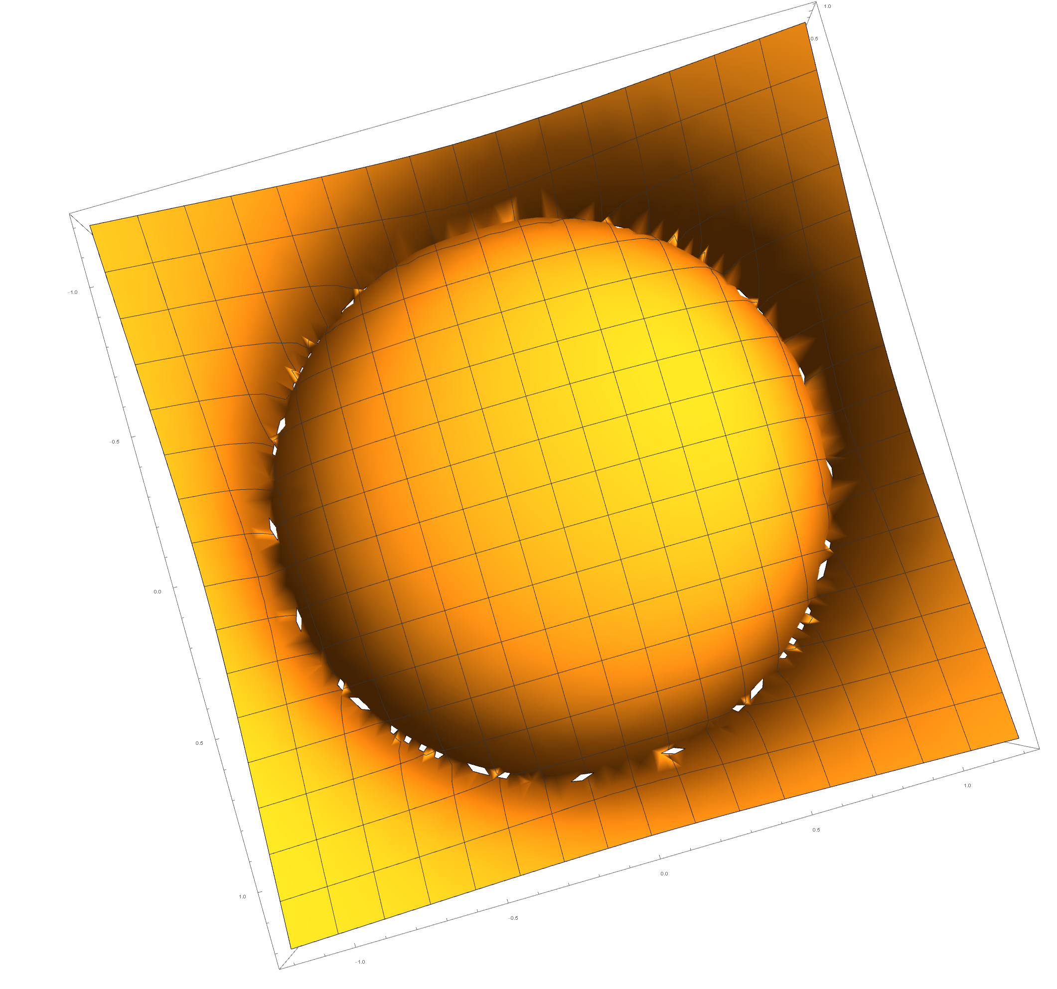
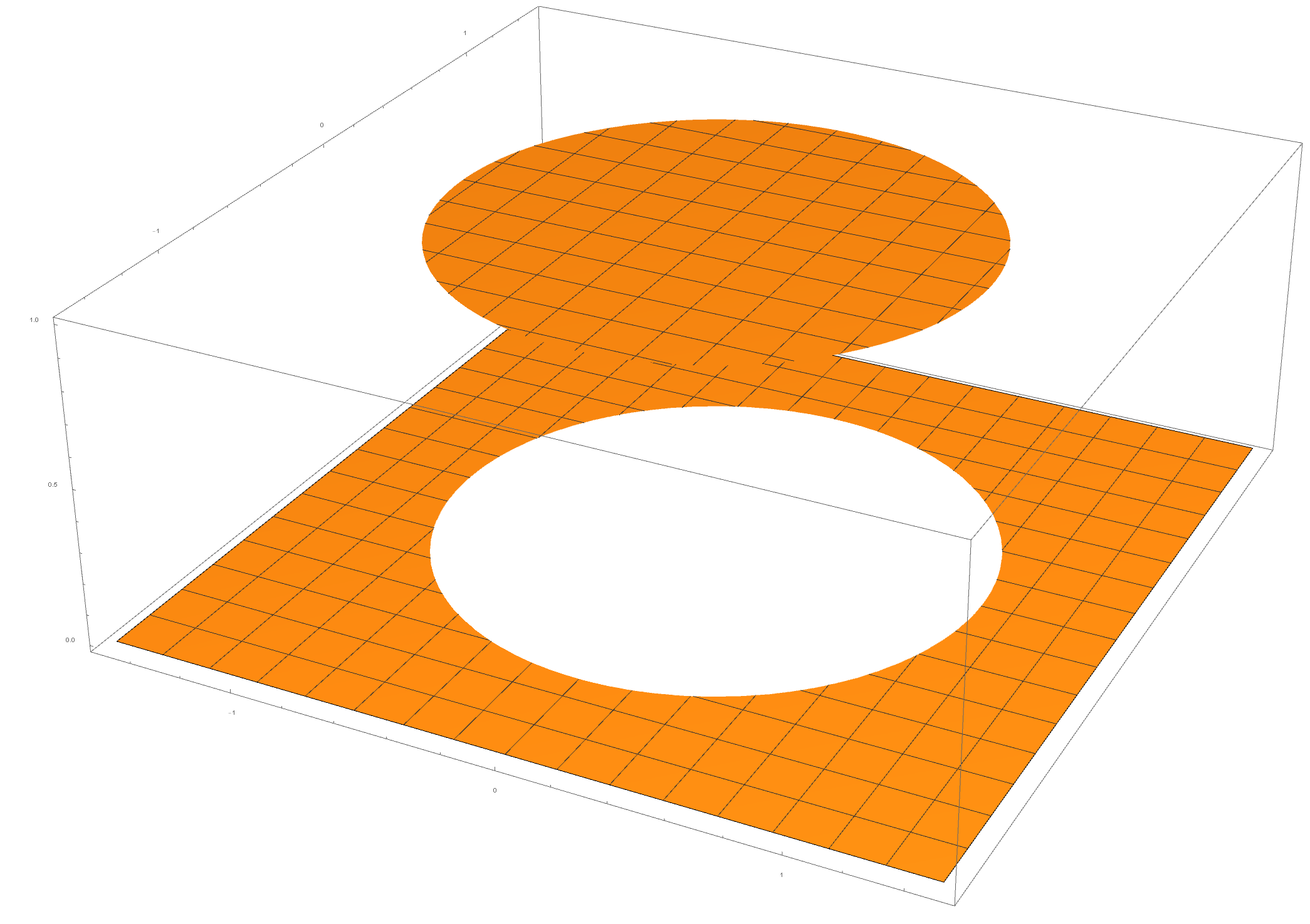
2.7. Surface Plot With Annular Edge

In example surface_plot_edge.cpp we had a surface plot with a large, undefined region easily discovered by Maple & Nathematica. In this example we have a surface with a smaller, annular undefined region that is harder for automatic software to get right. The function in question is as follows:

$\sqrt{\sqrt{| 1 - x^{2} - y^{2} |} - \frac{3}{20}}$

This example differs from surface_plot_edge.cpp in that we direct additional sampling near the unit circle. Other than that, it's just about identical.

MRPtree Version

Mathematica (from the side & top)

Paraview State File: https://github.com/richmit/MRPTree/blob/main/paraview/surface_plot_annular_edge.pvsm

XML VTK Data File: https://github.com/richmit/MRPTree/blob/main/paraview/surface_plot_annular_edge.vtu

Source code: https://github.com/richmit/MRPTree/blob/main/examples/surface_plot_annular_edge.cpp

#include "MR_rect_tree.hpp"
#include "MR_cell_cplx.hpp"
#include "MR_rt_to_cc.hpp"

typedef mjr::tree15b2d1rT            tt_t;
typedef mjr::MRccT5                  cc_t;
typedef mjr::MR_rt_to_cc<tt_t, cc_t> tc_t;

tt_t::rrpt_t annular_hat(tt_t::drpt_t xvec) {
  double v = std::sqrt(std::abs(1 - xvec[0] * xvec[0] - xvec[1] * xvec[1])) - 0.15;
  if (v < 0.0) {
    return std::numeric_limits<double>::quiet_NaN();
  } else {
    return std::sqrt(v);
  }
}

tt_t::src_t unit_circle_sdf(tt_t::drpt_t xvec) {
  double m = xvec[0] * xvec[0] + xvec[1] * xvec[1];
  return (1-m);
}

int main() {
  tt_t tree({-1.1, -1.1}, 
            { 1.1,  1.1});
  cc_t ccplx;

  // Sample a uniform grid across the domain
  tree.refine_grid(5, annular_hat);

  /* annular_hat produces NaNs in a thin annulus near the unit circle.*/
  tree.refine_leaves_recursive_cell_pred(7, annular_hat, [&tree](int i) { return (tree.cell_cross_sdf(i, unit_circle_sdf)); });

  /* Balance the three to the traditional level of 1 (no cell borders a cell more than half it's size) */
  tree.balance_tree(1, annular_hat);

  tree.dump_tree(10);

  /* By passing annular_hat() to the construct_geometry_fans() we enable broken edges (an edge with one good point and one NaN) to be repaired. */
  tc_t::construct_geometry_fans(ccplx,
                                tree,
                                2,
                                {{tc_t::val_src_spc_t::FDOMAIN, 0}, 
                                 {tc_t::val_src_spc_t::FDOMAIN, 1},
                                 {tc_t::val_src_spc_t::FRANGE,  0}},
                                annular_hat
                               );

  ccplx.create_named_datasets({"x", "y", "f(x,y)"},
                              {{"NORMALS", {0, 1, 2}}});

  ccplx.dump_cplx(10);

  ccplx.write_xml_vtk("surface_plot_annular_edge.vtu", "surface_plot_annular_edge");
}

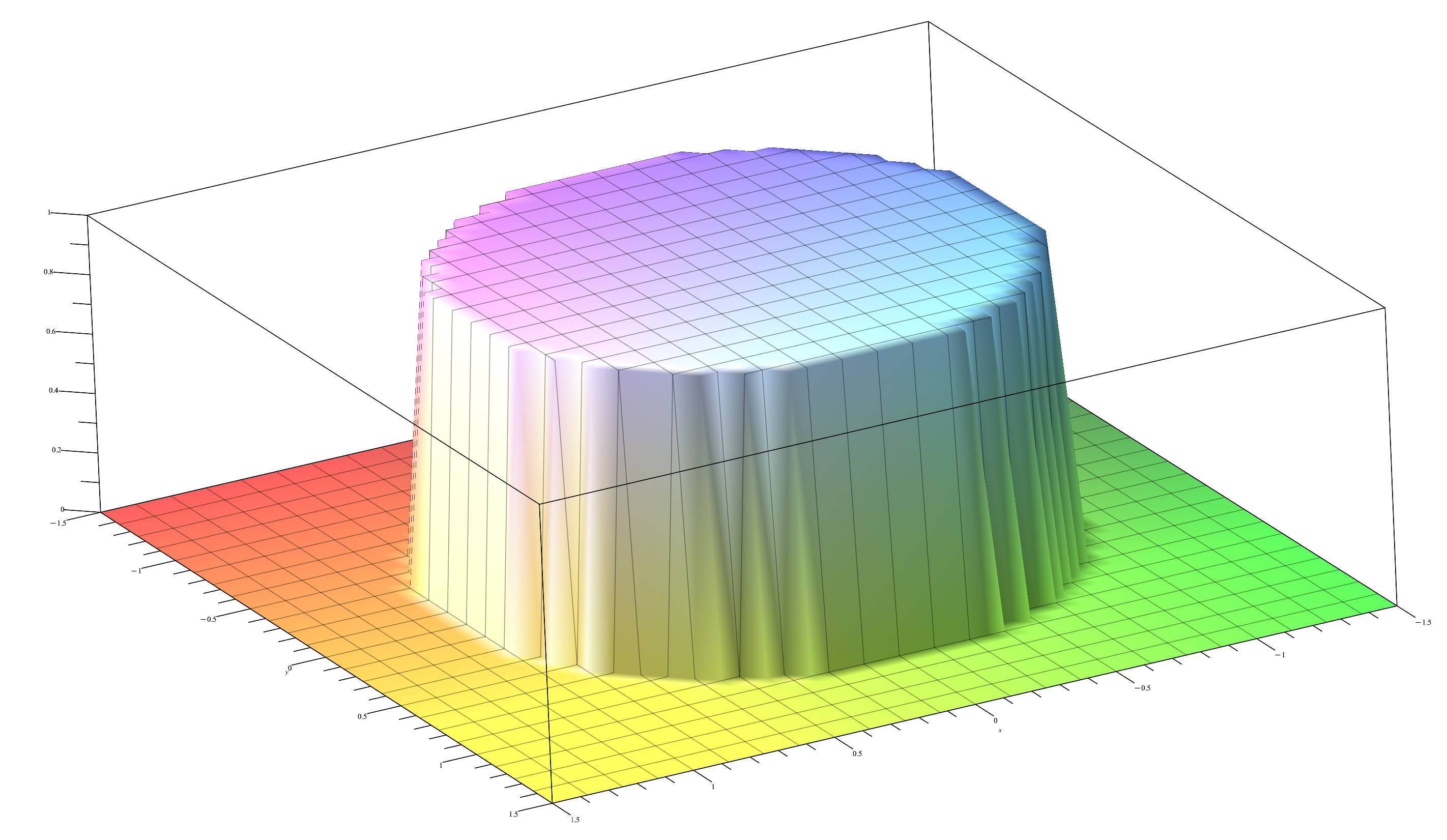
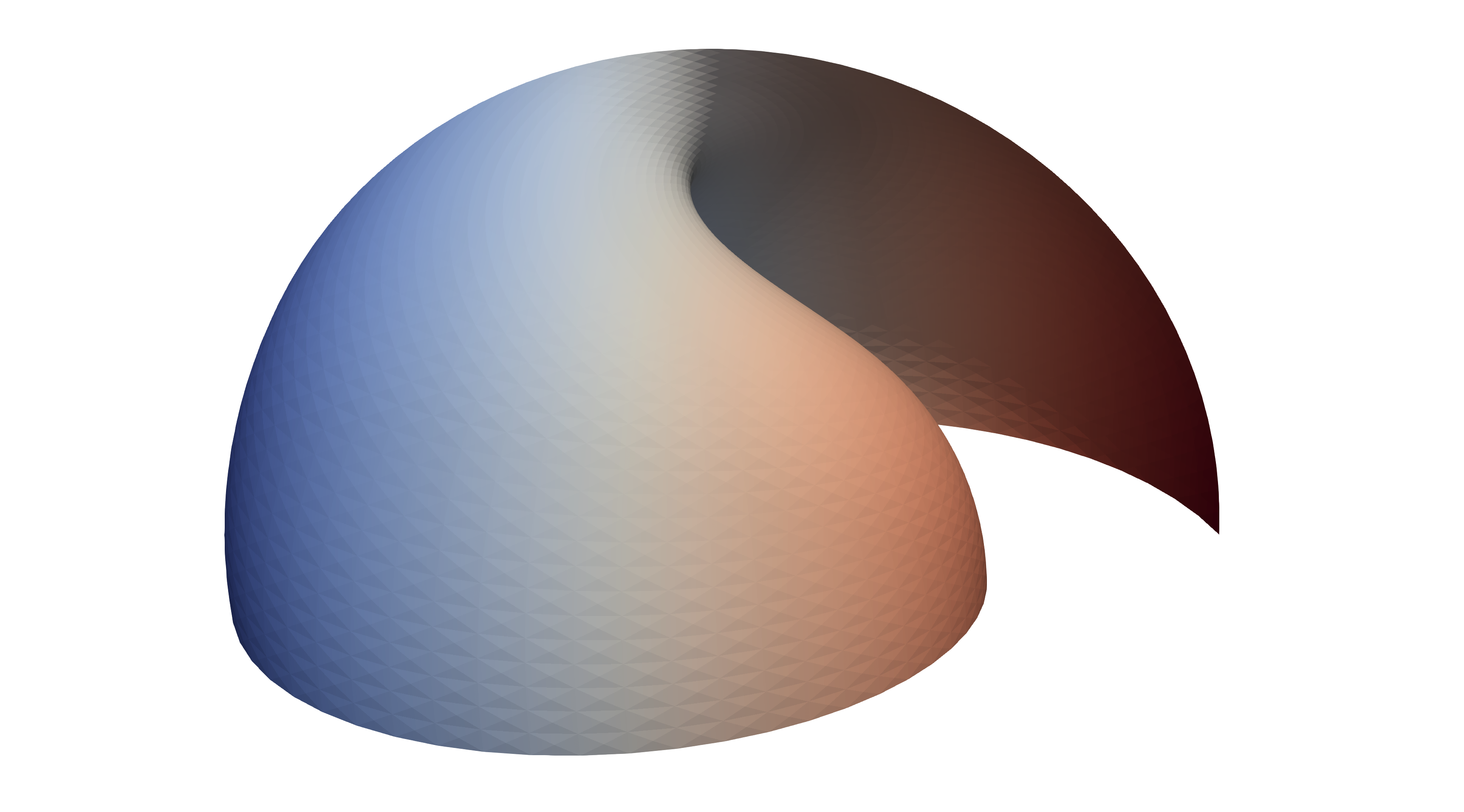
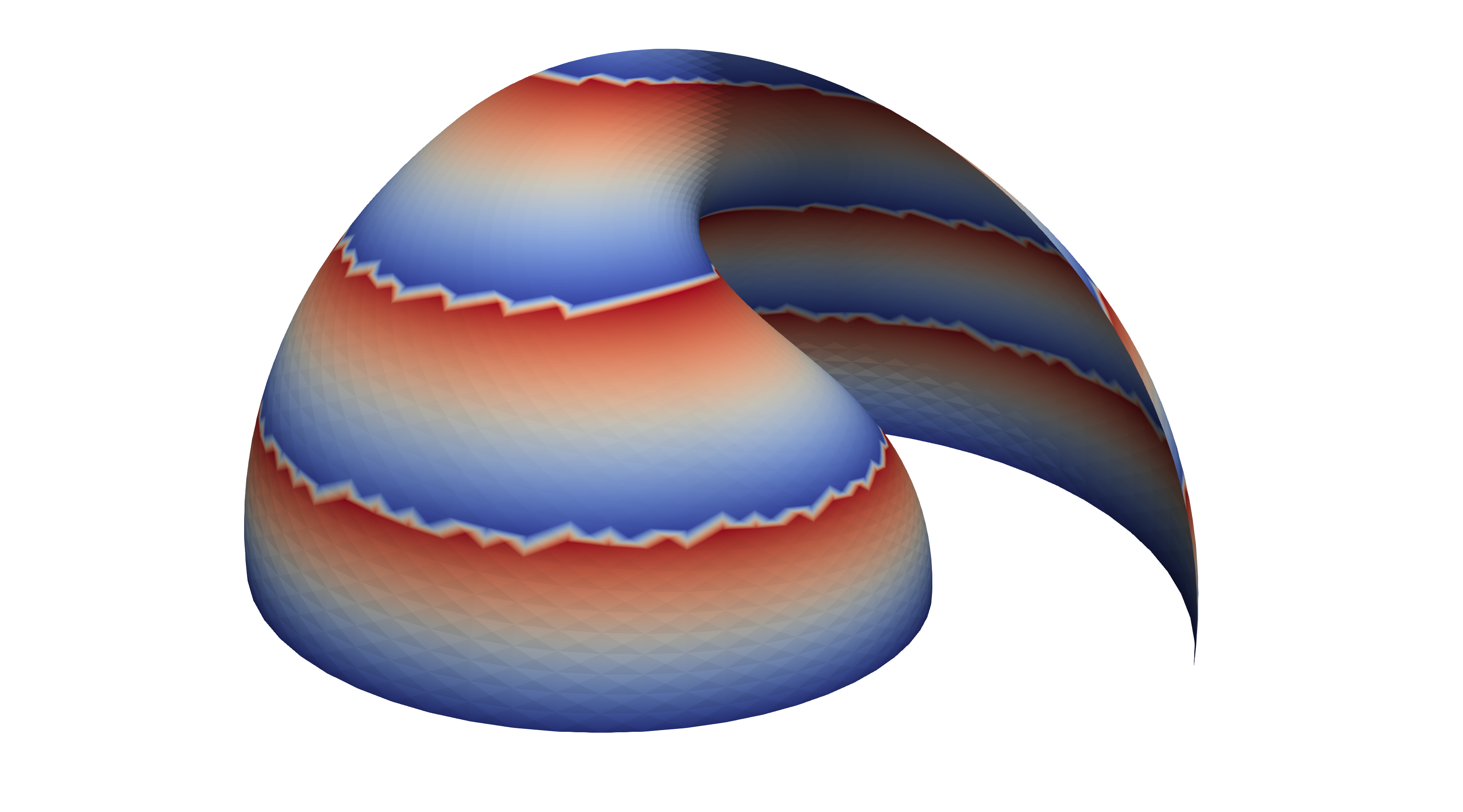
2.8. Surface Plot With An Corner

The function illustrated here is continuous on the entire plane, but has no derivative on the unit circle. While no derivative exists on the unit circle, directional derivatives pointing from the origin approach infinity as we get close to the unit circle. The derivative at the origin is zero. Thus the surface is not only zero on the unit circle, but it drops to zero very quickly from it's local extrema at the origin.

If we sample on a uniform grid, some of the resulting polygons will have vertexes both inside and outside the unit circle. These polygons will never touch the x-y plane, and thus the surface will not appear to have a uniform zero set on the unit circle. At low resolution the results are so bad they are difficult to interpret. At higher resolutions we see what appears to be a jagged edge over the unit circle. Meaning the results are visually quite wrong, but an astute viewer might well guess the true behavior of the function from the resulting image. In order to correct this graph we need sample points in the triangulation that are on, or very near, the unit circle. We can do that by folding and resampling the cell complex on the unit circle.

How to drive up the sample rate near a particular SDF – so that we get higher resolution where the surface meets the plane.
How to "fold" the resulting triangles to achieve higher accuracy on the non-differentiable edge.
How to use tsampf_to_cdatf() & tsdf_to_csdf() to adapt functions designed for a MR_rect_tree for use with a MR_cell_cplx.

Matlab 2023b & Mathematica 12 & Maple 2024.1

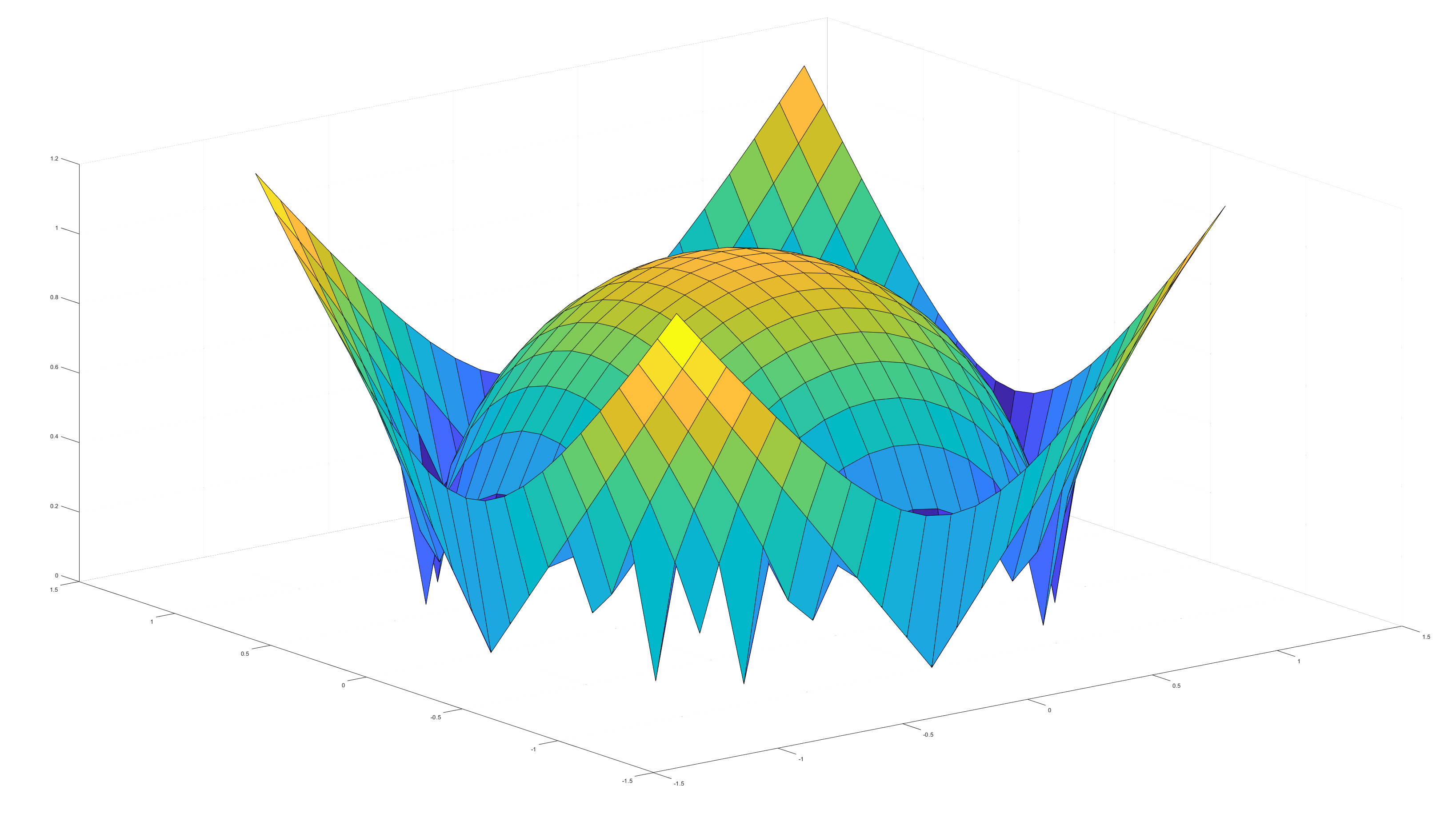
MRPtree Version

Paraview State File: https://github.com/richmit/MRPTree/blob/main/paraview/surface_plot_corner.pvsm

XML VTK Data File: https://github.com/richmit/MRPTree/blob/main/paraview/surface_plot_corner.vtu

Source code: https://github.com/richmit/MRPTree/blob/main/examples/surface_plot_corner.cpp

#include "MR_rect_tree.hpp"
#include "MR_cell_cplx.hpp"
#include "MR_rt_to_cc.hpp"

typedef mjr::tree15b2d1rT            tt_t;
typedef mjr::MRccT5                  cc_t;
typedef mjr::MR_rt_to_cc<tt_t, cc_t> tc_t;

tt_t::rrpt_t half_sphere_hat(tt_t::drpt_t xvec) {
  double m = xvec[0] * xvec[0] + xvec[1] * xvec[1];
  return (std::sqrt(std::abs(1-m)));
}

tt_t::src_t unit_circle_sdf(tt_t::drpt_t xvec) {
  double m = xvec[0] * xvec[0] + xvec[1] * xvec[1];
  return (1-m);
}

int main() {
  tt_t tree({-1.1, -1.1}, 
            { 1.1,  1.1});
  cc_t ccplx;

  /* Here is another way to get fine samples on the circle, but with a SDF this time. */
  tree.refine_grid(5, half_sphere_hat);

  /* Increase sample resolution on the unit circle.  Here we do that with an SDF. */
  tree.refine_leaves_recursive_cell_pred(7, half_sphere_hat, [&tree](int i) { return (tree.cell_cross_sdf(i, unit_circle_sdf)); });

  /* Balance the three to the traditional level of 1 (no cell borders a cell more than half it's size) */
  tree.balance_tree(1, half_sphere_hat);

  /* Take a peek at the raw tree data */
  tree.dump_tree(10);

  /* Generate a cell complex from the tree samples */
  tc_t::construct_geometry_fans(ccplx,
                                tree,
                                2,
                                {{tc_t::val_src_spc_t::FDOMAIN, 0}, 
                                 {tc_t::val_src_spc_t::FDOMAIN, 1},
                                 {tc_t::val_src_spc_t::FRANGE,  0}});

  /* The single argument form of create_named_datasets() allows us to easily name data points. */
  ccplx.create_named_datasets({"x", "y", "f(x,y)"});

  /* Take a look at the generated cell complex */
  ccplx.dump_cplx(10);

  /* Fold all triangles that cross the unit circle! */
  ccplx.triangle_folder([](cc_t::node_data_t x){return tc_t::tsampf_to_cdatf(half_sphere_hat, x); }, 
                        [](cc_t::node_data_t x){return tc_t::tsdf_to_csdf(unit_circle_sdf,    x); });

  /* Notice how it changed after the fold */
  ccplx.dump_cplx(10);

  ccplx.write_xml_vtk("surface_plot_corner.vtu", "surface_plot_corner");
}

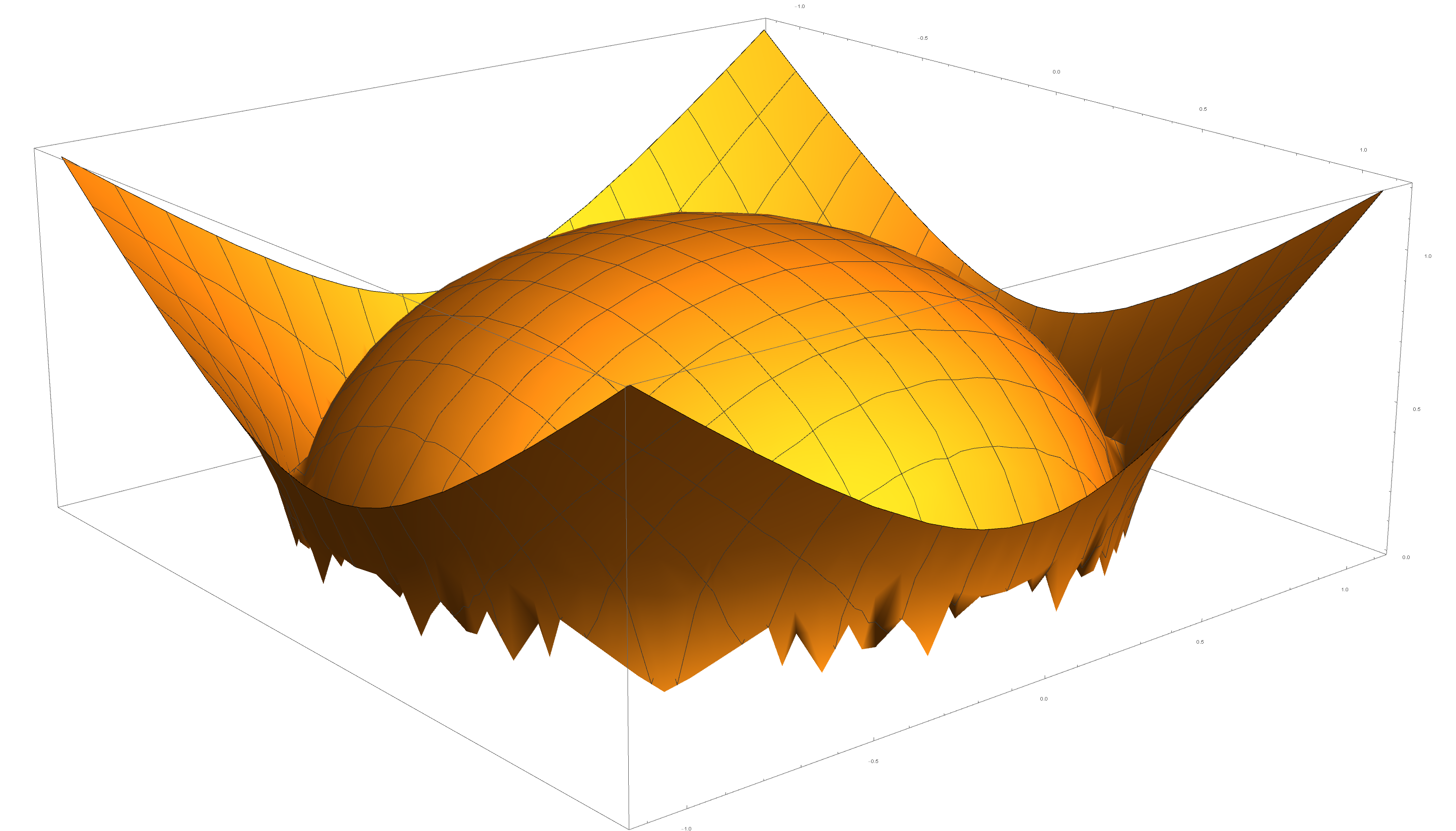
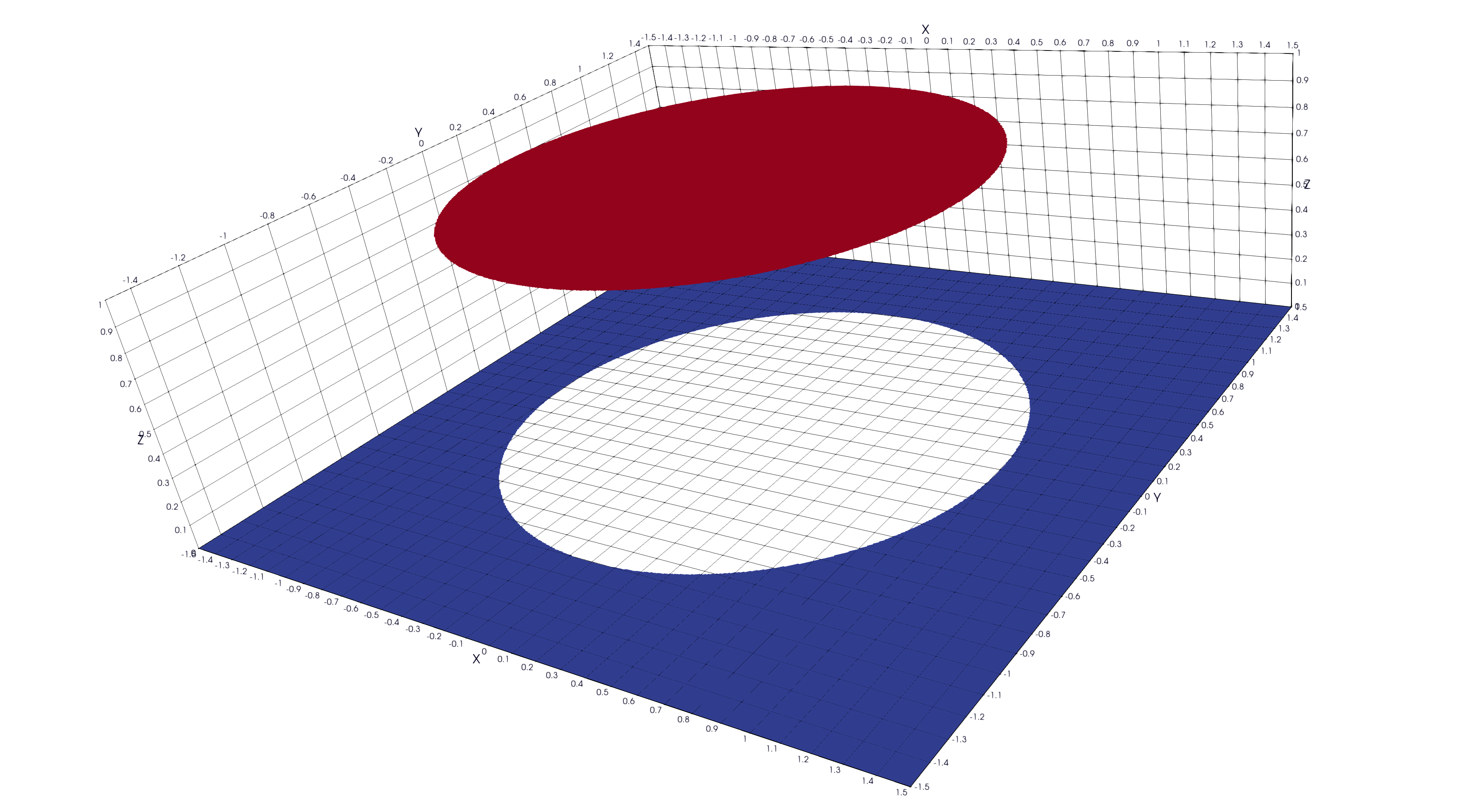
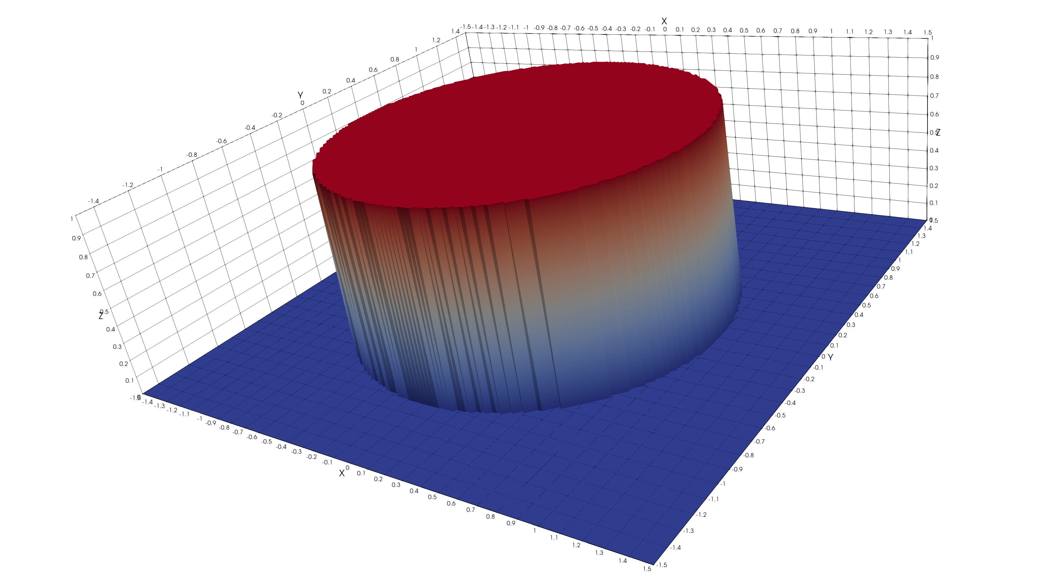
2.9. Surface Plot With An Step

The function illustrated here is defined on the entire plan, but has a step discontinuity on the unit circle. Except on the unit circle, the function's derivative is zero. If we sample on a uniform grid, some of the resulting polygons will have vertexes both inside and outside the unit circle – they cross over the discontinuity! When drawn we get a continuous surface with a circular bump! It should look like the x-y plane has a circle cut out that is hovering one unit above the plane.

How to drive up the sample rate near a particular SDF – so that we get higher resolution where the surface meets the plane.
How to delete triangles that cross over a discontinuity – via an SDF.

MRPtree (with & without cut)

Mathematica 12 & Maple 2024.1

Source code: https://github.com/richmit/MRPTree/blob/main/examples/surface_plot_step.cpp

#include "MR_rect_tree.hpp"
#include "MR_cell_cplx.hpp"
#include "MR_rt_to_cc.hpp"

typedef mjr::tree15b2d1rT            tt_t;
typedef mjr::MRccT5                  cc_t;
typedef mjr::MR_rt_to_cc<tt_t, cc_t> tc_t;

tt_t::rrpt_t hover_circle(tt_t::drpt_t xvec) {
  return (xvec[0] * xvec[0] + xvec[1] * xvec[1] < 1);
}

tt_t::src_t unit_circle_sdf(tt_t::drpt_t xvec) {
  double m = xvec[0] * xvec[0] + xvec[1] * xvec[1];
  return (1-m);
}

int main() {
  tt_t tree({-1.5, -1.5}, 
            { 1.5,  1.5});
  cc_t ccplx;

  /* Here is another way to get fine samples on the circle, but with a SDF this time. */
  tree.refine_grid(5, hover_circle);

  /* Increase sample resolution on the unit circle.  Here we do that with an SDF. */
  tree.refine_leaves_recursive_cell_pred(7, hover_circle, [&tree](int i) { return (tree.cell_cross_sdf(i, unit_circle_sdf)); });

  /* Balance the three to the traditional level of 1 (no cell borders a cell more than half it's size) */
  tree.balance_tree(1, hover_circle);

  /* Take a peek at the raw tree data */
  tree.dump_tree(10);

  /* Generate a cell complex from the tree samples */
  tc_t::construct_geometry_fans(ccplx,
                                tree,
                                2,
                                {{tc_t::val_src_spc_t::FDOMAIN, 0}, 
                                 {tc_t::val_src_spc_t::FDOMAIN, 1},
                                 {tc_t::val_src_spc_t::FRANGE,  0}});

  /* The single argument form of create_named_datasets() allows us to easily name data points. */
  ccplx.create_named_datasets({"x", "y", "f(x,y)"});

  /* Take a look at the generated cell complex */
  ccplx.dump_cplx(10);

  /* Cut out the tiny triangles on the unit circle! */
  tc_t::cull_cc_cells_on_domain_sdf_boundry(ccplx, unit_circle_sdf);

  /* We can do the above directly with MR_cell_cplx::cull_cells().  If you rewrote unit_circle_sdf(), you don't need to nest lambdas... */
  // ccplx.cull_cells([&ccplx](cc_t::cell_verts_t c){ return ccplx.cell_cross_sdf_boundry(c, 
  //                                                                                [](cc_t::node_data_t pd) { return (tc_t::tsdf_to_csdf(unit_circle_sdf, 
  //                                                                                                                                     pd)); 
  //                                                                                                        }); 
  //                                          });

  /* Notice how it changed after the fold */
  ccplx.dump_cplx(10);

  ccplx.write_xml_vtk("surface_plot_step.vtu", "surface_plot_step");
}

2.10. Surface Branches & Glue

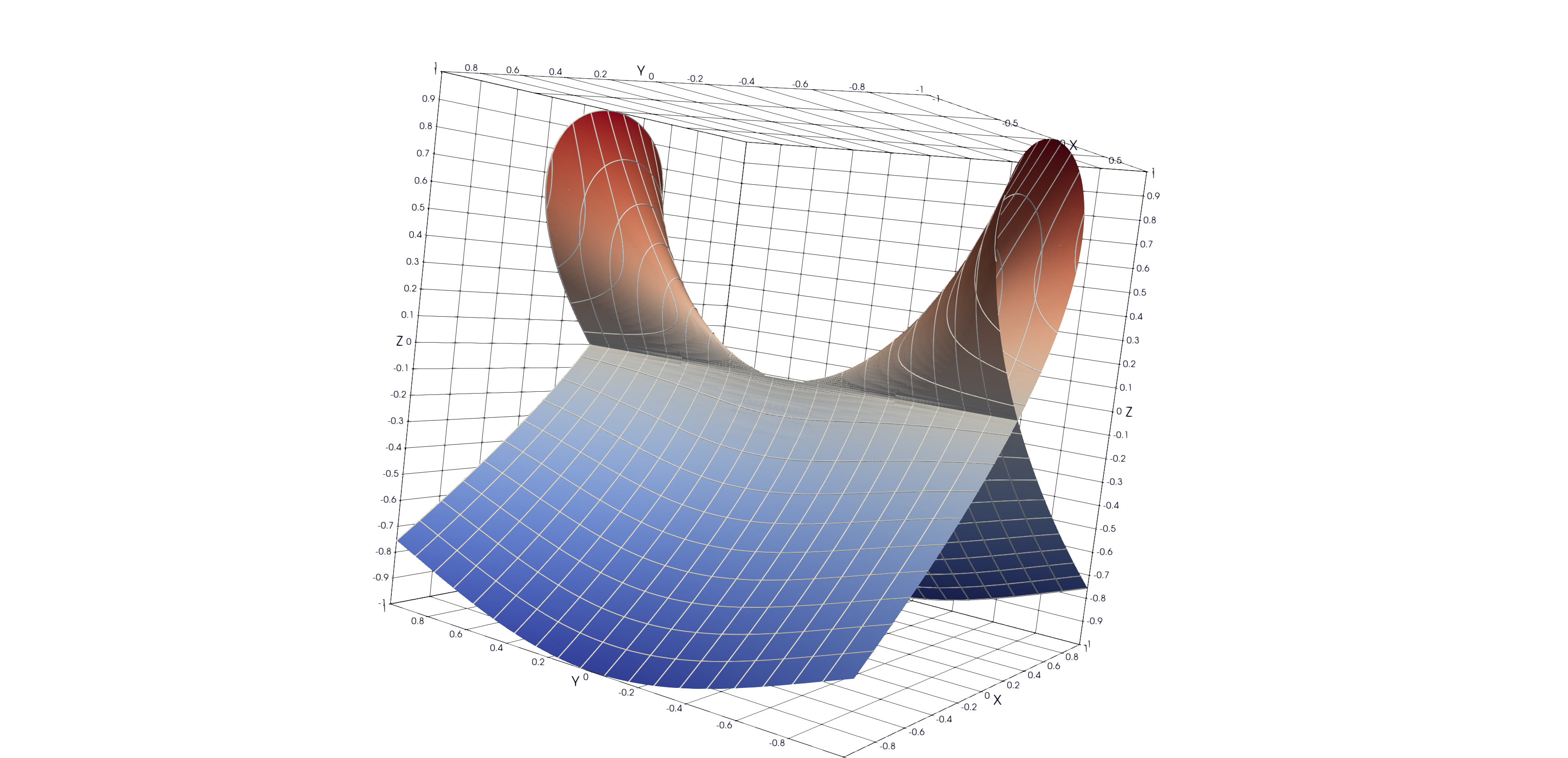
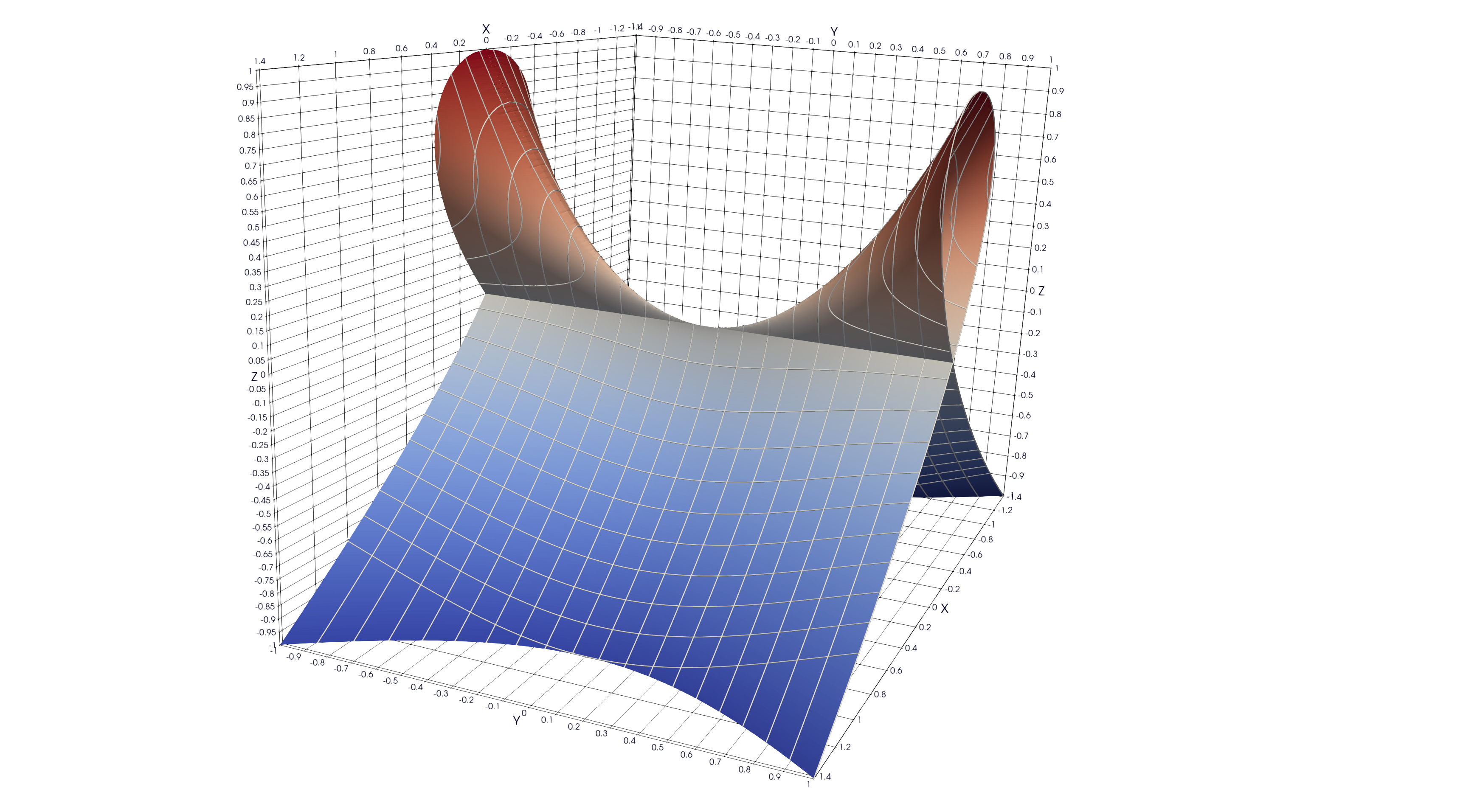
In surface_plot_edge.cpp we encountered the unit sphere defined by the zeros of $1^{2} = x^{2} + y^{2} + z^{2}$ , and the related function $f (x, y) = \sqrt{1 - x^{2} - y^{2}}$ obtained by "solving" for $z$ . Note that if $z = f (x, y)$ , then both $z$ and $- z$ satisfy the original equation. While the square root function is positive by definition, we might wish to think of $f (x, y)$ as a multi-valued function with two branches – a positive one and a negative one.

In simple cases like this, where the two branches are reflections across an axis plane, we can use MR_cell_cplx::mirror() to mirror the geometry and seal up any holes. This is really the only change from surface_plot_edge.cpp.

Paraview State File: https://github.com/richmit/MRPTree/blob/main/paraview/surface_branch_glue.pvsm

XML VTK Data File: https://github.com/richmit/MRPTree/blob/main/paraview/surface_branch_glue.vtu

Source code: https://github.com/richmit/MRPTree/blob/main/examples/surface_branch_glue.cpp

#include "MR_rect_tree.hpp"
#include "MR_cell_cplx.hpp"
#include "MR_rt_to_cc.hpp"

typedef mjr::tree15b2d1rT            tt_t;
typedef mjr::MRccT5                  cc_t;
typedef mjr::MR_rt_to_cc<tt_t, cc_t> tc_t;

tt_t::rrpt_t half_sphere(tt_t::drpt_t xvec) {
  double m = xvec[0] * xvec[0] + xvec[1] * xvec[1];
  if (m > 1) {
    return std::numeric_limits<double>::quiet_NaN();
  } else {
    return std::sqrt(1-m);
  }
}

int main() {
  tt_t tree({-1.2, -1.2}, 
            { 1.2,  1.2});
  cc_t ccplx;

  // Sample a uniform grid across the domain
  tree.refine_grid(5, half_sphere);

  /* Refine near the edge */
  tree.refine_recursive_if_cell_vertex_is_nan(6, half_sphere);

  tree.dump_tree(10);

  /* By passing half_sphere() to the construct_geometry_fans() we enable broken edges (an edge with one good point and one NaN) to be repaired. */
  tc_t::construct_geometry_fans(ccplx,
                                tree,
                                2,
                                {{tc_t::val_src_spc_t::FDOMAIN, 0}, 
                                 {tc_t::val_src_spc_t::FDOMAIN, 1},
                                 {tc_t::val_src_spc_t::FRANGE,  0}},
                                half_sphere
                               );

  ccplx.create_named_datasets({"x", "y", "f(x,y)"},
                              {{"NORMALS", {0, 1, 2}}});

  /* This is the magic.  We add new cells with the third element of each point data vector negated. */
  ccplx.mirror({0, 0, 1});

  ccplx.dump_cplx(10);

  ccplx.write_xml_vtk("surface_branch_glue.vtu", "surface_branch_glue");
  ccplx.write_legacy_vtk("surface_branch_glue.vtk", "surface_branch_glue");
  ccplx.write_ply("surface_branch_glue.ply", "surface_branch_glue");
}

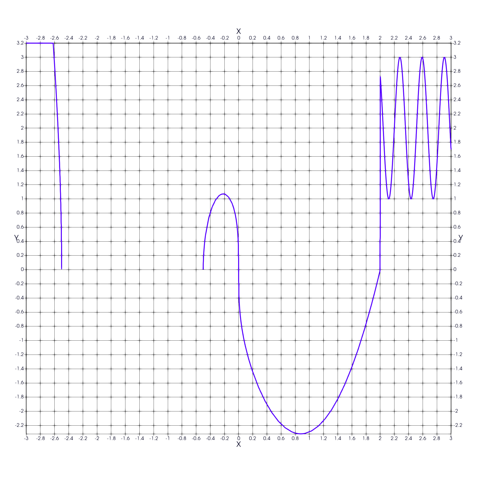
2.11. Curve Plot

Univariate function plots are the bread-and-butter of the plotting world. Normally a simple, uniformly spaced, sequence is enough to get the job done quite nicely. Still, a few things can come up:

Jump discontinuities & Vertical asymptotes: Resolved with higher sampling near the discontinuities and a cutting edge (TBD)
Isolated, non-differentiable points: Resolved with higher sampling near the points and a folding edge (TBD)
Undefined intervals: Resolved with higher sampling near the edges and NaN edge repair
Regions of high oscillation: Resolved with higher sampling on the regions
Extrema: Resolved with higher sampling near the extrema

Note that most of the items above are listed TBD. A few features need to be added to MR_rt_to_cc. ;) Note the TODO comments in the body of main().

Paraview State File: https://github.com/richmit/MRPTree/blob/main/paraview/curve_plot.pvsm

XML VTK Data File: https://github.com/richmit/MRPTree/blob/main/paraview/curve_plot.vtu

Source code: https://github.com/richmit/MRPTree/blob/main/examples/curve_plot.cpp

#include "MR_rect_tree.hpp"
#include "MR_cell_cplx.hpp"
#include "MR_rt_to_cc.hpp"

typedef mjr::tree15b1d1rT            tt_t;
typedef mjr::MRccT5                  cc_t;
typedef mjr::MR_rt_to_cc<tt_t, cc_t> tc_t;

tt_t::rrpt_t f(tt_t::drpt_t x) { 
  double ret = (x<0?-1:1)*std::pow(std::abs(x), 1/3.0) * std::sqrt((x+1.5)*(x+1.5)-1) * (x-2);
  if (x>2)
    ret = 2+std::sin(20*x);
  if (ret < -3)
    ret = -3;
  if (ret > 3.2)
    ret = 3.2;
  return ret;
}

int main() {
  tt_t tree(-3, 3);
  cc_t ccplx;

  // Sample a uniform grid across the domain
  tree.refine_grid(5, f);

  // Refine near NaN
  tree.refine_recursive_if_cell_vertex_is_nan(10, f);
  // TODO: Add NaN edge repair when implemented in MR_rt_to_cc

  // Refine near vertical tangent line
  tree.refine_leaves_recursive_cell_pred(10, f, [&tree](tt_t::diti_t i) { return (tree.cell_close_to_domain_point(0.0, 1.0e-2, i)); });
  // TODO: Use derivative test for this

  // Step discontinuities at 2.
  tree.refine_leaves_recursive_cell_pred(10, f, [&tree](tt_t::diti_t i) { return (tree.cell_close_to_domain_point(2.0, 1.0e-2, i)); });
  // TODO: Add cell cut when implemented in MR_rt_to_cc

  // Non differentiable point near x=-2.619185320
  tree.refine_leaves_recursive_cell_pred(11, f, [&tree](tt_t::diti_t i) { return (tree.cell_close_to_domain_point(-2.619185320, 1.0e-2, i)); });
  // TODO: Add folding edge when implemented in MR_rt_to_cc

  // High oscillation from [2,3]
  tree.refine_leaves_recursive_cell_pred(10, f, [&tree](tt_t::diti_t i) { return (tree.diti_to_drpt(i) >= 2.0); });

  // Extrema near -0.2171001290
  tree.refine_leaves_recursive_cell_pred(10, f, [&tree](tt_t::diti_t i) { return (tree.cell_close_to_domain_point(-0.2171001290, 1.0e-2, i)); });
  // TODO: Use derivative test for this

  // Extrema near 0.8775087009
  tree.refine_leaves_recursive_cell_pred(8, f, [&tree](tt_t::diti_t i) { return (tree.cell_close_to_domain_point(0.8775087009, 1.0e-2, i)); });
  // TODO: Use derivative test for this

  tree.dump_tree(10);

  tc_t::construct_geometry_fans(ccplx,
                                tree,
                                1,
                                {{tc_t::val_src_spc_t::FDOMAIN,   0  }, 
                                 {tc_t::val_src_spc_t::FRANGE,    0  },
                                 {tc_t::val_src_spc_t::CONSTANT, 0.0}},
                                f
                               );

  // Note the first argument need not name *every* data element, just the first ones.
  ccplx.create_named_datasets({"x", "f(x)"});

  ccplx.dump_cplx(10);

  ccplx.write_xml_vtk("curve_plot.vtu", "curve_plot");
}

2.12. Parametric Surface With Defects

This example illustrates some of the things that can go wrong when generating parametric surfaces. We dump two version of the tessellation – one with quads and one with triangles. This allows us to better illustrate how some defects show up.

Quads that are not plainer. Look closely at the rectangular tessellation, and note the "rectangles" appear to be broken in across the diagonal – at least that's how they appear in most tools including Paraview & meshlab.
At the poles, the rectangular cells of the tree map to three distinct points instead of four. This means for the rectangular tessellation, the rectangles at the poles are degenerate! Then converting from tree to cell complex, these quads are removed because they are degenerate. This is not an issue for the triangular tessellation (FANS).
The v=0 edge meets up with the v=1 edge. Because we have chk_point_unique set to true for the cell complex object, the duplicate points are "welded" together when the points are added. This results in a seamless edge.

Paraview State File: https://github.com/richmit/MRPTree/blob/main/paraview/parametric_surface_with_defects.pvsm

XML VTK Data File 1: https://github.com/richmit/MRPTree/blob/main/paraview/parametric_surface_with_defects-tri.vtu

XML VTK Data File 2: https://github.com/richmit/MRPTree/blob/main/paraview/parametric_surface_with_defects-rect.vtu

Source code: https://github.com/richmit/MRPTree/blob/main/examples/parametric_surface_with_defects.cpp

#include <numbers>                                                       /* C++ math constants      C++20    */

#include "MR_rect_tree.hpp"
#include "MR_cell_cplx.hpp"
#include "MR_rt_to_cc.hpp"

typedef mjr::tree15b2d3rT            tt_t;
typedef mjr::MRccT5                  cc_t;
typedef mjr::MR_rt_to_cc<tt_t, cc_t> tc_t;

tt_t::rrpt_t par_sphere(tt_t::drpt_t xvec) {
  double u = std::numbers::pi/4 * xvec[0] + std::numbers::pi/4;
  double v = std::numbers::pi   * xvec[1] + std::numbers::pi;
  return { std::sin(u)*std::cos(v),
           std::sin(u)*std::sin(v),
           std::cos(u)
         };
}                          

int main() {
  tt_t tree;
  cc_t ccplx;

  /* Uniform sampling */
  tree.refine_grid(6, par_sphere);

  /* First we dump a tessellation made of triangles */
  tc_t::construct_geometry_fans(ccplx,
                                tree,
                                2,
                                {{tc_t::val_src_spc_t::FRANGE, 0},
                                 {tc_t::val_src_spc_t::FRANGE, 1},
                                 {tc_t::val_src_spc_t::FRANGE, 2}});
  ccplx.create_named_datasets({"u", "v", "x(u,v)", "y(u,v)", "z(u,v)"});
  ccplx.dump_cplx(5);
  ccplx.write_xml_vtk("parametric_surface_with_defects-tri.vtu", "parametric_surface_with_defects-tri");

  /* Next we dump a tessellation made of rectangles */
  ccplx.clear(); // We need to clear out the old contents first!
  tc_t::construct_geometry_rects(ccplx,
                                 tree,
                                 2,
                                 {{tc_t::val_src_spc_t::FRANGE, 0},
                                  {tc_t::val_src_spc_t::FRANGE, 1},
                                  {tc_t::val_src_spc_t::FRANGE, 2}});
  ccplx.create_named_datasets({"u", "v", "x(u,v)", "y(u,v)", "z(u,v)"});
  ccplx.dump_cplx(5);
  ccplx.write_xml_vtk("parametric_surface_with_defects-rect.vtu", "parametric_surface_with_defects-rect");
}

2.13. High Resolution Parametric Surface

Just a nice parametric surface without any weirdness. Some things demonstrated:

How to time various operations.
- Try with a large mesh (use a 9 in refine_grid).
- Try reducing the number of data variables stored in the cell complex
- Try removing the normal vector from the output
- Try both MRccT5 & MRccF5 for cc_t
How to include a synthetic value that can be used for color mapping – c(u,v) can be used to render stripes on the surface.
How to compute a normal to a parametric surface
How to include a normal in the cell complex

Surfaces with and without normals

Stripes!!

Paraview State File: https://github.com/richmit/MRPTree/blob/main/paraview/performance_with_large_surface.pvsm

XML VTK Data File: https://github.com/richmit/MRPTree/blob/main/paraview/performance_with_large_surface.vtu

Source code: https://github.com/richmit/MRPTree/blob/main/examples/performance_with_large_surface.cpp

#include <chrono>                                                        /* time                    C++11    */
#include <numbers>                                                       /* C++ math constants      C++20    */

#include "MR_rect_tree.hpp"
#include "MR_cell_cplx.hpp"
#include "MR_rt_to_cc.hpp"

typedef mjr::tree15b2d15rT           tt_t;
typedef mjr::MRccT5                  cc_t;   // Replace with mjr::MRccF5, and compare bridge performance.
typedef mjr::MR_rt_to_cc<tt_t, cc_t> tc_t;

tt_t::rrpt_t stripy_shell(tt_t::drpt_t xvec) {
  double u    = std::numbers::pi   * xvec[0] + std::numbers::pi + 0.1; // U transformed from unit interval
  double v    = std::numbers::pi/2 * xvec[1] + std::numbers::pi/2;     // V transformed from unit interval
  double x    = u*std::sin(u)*std::cos(v);                             // X
  double y    = u*std::cos(u)*std::cos(v);                             // Y
  double z    = u*std::sin(v);                                         // Z
  double c    = std::fmod(u*sin(v), 2);                                // Stripes
  double dxdu = std::sin(u)*std::cos(v)+u*std::cos(u)*std::cos(v);     // dX/du
  double dxdv = -u*std::sin(u)*std::sin(v);                            // dX/dv
  double dydu = std::cos(u)*std::cos(v)-u*std::sin(u)*std::cos(v);     // dY/du
  double dydv = -u*std::cos(u)*std::sin(v);                            // dY/dv
  double dzdu = std::sin(v);                                           // dZ/du
  double dzdv = u*std::cos(v);                                         // dZ/dv
  double nx   = dydu*dzdv-dydv*dzdu;                                   // normal_X     This noraml      
  double ny   = dxdv*dzdu-dxdu*dzdv;                                   // normal_Y     will not be of 
  double nz   = dxdu*dydv-dxdv*dydu;                                   // normal_Z     unit length
  return {x, y, z, c, dxdu, dxdv, dydu, dydv, dzdu, dzdv, nx, ny, nz};
}                          

int main() {
  std::chrono::time_point<std::chrono::system_clock> start_time = std::chrono::system_clock::now();
  tt_t tree;
  cc_t ccplx;
  std::chrono::time_point<std::chrono::system_clock> construct_time = std::chrono::system_clock::now();

  tree.refine_grid(7, stripy_shell);
  std::chrono::time_point<std::chrono::system_clock> sample_time = std::chrono::system_clock::now();

  tree.dump_tree(10);
  std::chrono::time_point<std::chrono::system_clock> tdump_time = std::chrono::system_clock::now();

  tc_t::construct_geometry_fans(ccplx,
                                tree,
                                2,
                                {{tc_t::val_src_spc_t::FRANGE,  0},
                                 {tc_t::val_src_spc_t::FRANGE,  1},
                                 {tc_t::val_src_spc_t::FRANGE,  2}});
  std::chrono::time_point<std::chrono::system_clock> fan_time = std::chrono::system_clock::now();

  ccplx.create_named_datasets({"u", "v", 
                               "x(u,v)", "y(u,v)", "z(u,v)",
                               "c(u,v)", 
                               "dx(u,v)/du", "dx(u,v)/dv", "dy(u,v)/du", "dy(u,v)/dv", "dz(u,v)/du", "dz(u,v)/dv",
                               "nx", "ny", "nz"}, 
                              {{"NORMALS", {12, 13, 14}}});
  std::chrono::time_point<std::chrono::system_clock> dat_anno_time = std::chrono::system_clock::now();

  ccplx.dump_cplx(10);
  std::chrono::time_point<std::chrono::system_clock> cdump_time = std::chrono::system_clock::now();

  ccplx.write_xml_vtk("performance_with_large_surface.vtu", "performance_with_large_surface");
  std::chrono::time_point<std::chrono::system_clock> write_time = std::chrono::system_clock::now();

  std::cout << "construct_time time .. " << static_cast<std::chrono::duration<double>>(construct_time-start_time)   << " sec" << std::endl;
  std::cout << "sample_time time ..... " << static_cast<std::chrono::duration<double>>(sample_time-construct_time)  << " sec" << std::endl;
  std::cout << "tree dump time ....... " << static_cast<std::chrono::duration<double>>(tdump_time-sample_time)      << " sec" << std::endl;
  std::cout << "bridge time .......... " << static_cast<std::chrono::duration<double>>(fan_time-tdump_time)         << " sec" << std::endl;
  std::cout << "dataset anno time .... " << static_cast<std::chrono::duration<double>>(dat_anno_time-fan_time)      << " sec" << std::endl;
  std::cout << "complex dump time .... " << static_cast<std::chrono::duration<double>>(cdump_time-dat_anno_time)    << " sec" << std::endl;
  std::cout << "write_vtk time ....... " << static_cast<std::chrono::duration<double>>(write_time-cdump_time)       << " sec" << std::endl;
  std::cout << "Total Run _time ...... " << static_cast<std::chrono::duration<double>>(write_time-start_time)       << " sec" << std::endl;
}

3. Extra Examples

The examples that follow are mostly just interesting mathematical objects. No new MRPTree functionality is demonstrated beyond what is demonstrated in the core examples.

3.1. Trefoil Parametric Surface

This example doesn't really demonstrate anything not found in the other examples. It's just a neat surface. ;)

Source code: https://github.com/richmit/MRPTree/blob/main/examples/trefoil.cpp

#include <numbers>                                                       /* C++ math constants      C++20    */

#include "MR_rect_tree.hpp"
#include "MR_cell_cplx.hpp"
#include "MR_rt_to_cc.hpp"

typedef mjr::tree15b2d6rT            tt_t;
typedef mjr::MRccT5                  cc_t;
typedef mjr::MR_rt_to_cc<tt_t, cc_t> tc_t;

tt_t::rrpt_t trefoil(tt_t::drpt_t xvec) {
  double u = xvec[0] * std::numbers::pi;
  double v = xvec[1] * std::numbers::pi;
  double r = 5;
  double x = r * std::sin(3 * u) / (2 + std::cos(v));
  double y = r * (std::sin(u) + 2 * std::sin(2 * u)) / (2 + std::cos(v + std::numbers::pi * 2 / 3));
  double z = r / 2 * (std::cos(u) - 2 * std::cos(2 * u)) * (2 + std::cos(v)) * (2 + std::cos(v + std::numbers::pi * 2 / 3)) / 4;
  double dxdu = (3*r*std::cos(3*u))/(std::cos(v)+2);
  double dxdv = (r*std::sin(3*u)*std::sin(v))/(std::cos(v)+2)/(std::cos(v)+2);
  double dydu = (r*(4*std::cos(2*u)+std::cos(u)))/(std::cos(v+(2*std::numbers::pi)/3)+2);
  double dydv = (r*(2*std::sin(2*u)+std::sin(u))*std::sin(v+(2*std::numbers::pi)/3))/
    ((std::cos(v+(2*std::numbers::pi)/3)+2)*(std::cos(v+(2*std::numbers::pi)/3)+2));
  double dzdu = (r*(4*std::sin(2*u)-std::sin(u))*(std::cos(v)+2)*(std::cos(v+(2*std::numbers::pi)/3)+2))/8;
  double dzdv = (-(r*(std::cos(u)-2*std::cos(2*u))*(std::cos(v)+2)*std::sin(v+(2*std::numbers::pi)/3))/8) -
    (r*(std::cos(u)-2*std::cos(2*u))*std::sin(v)*(std::cos(v+(2*std::numbers::pi)/3)+2))/8;
  double nx   = dydu*dzdv-dydv*dzdu;
  double ny   = dxdv*dzdu-dxdu*dzdv;
  double nz   = dxdu*dydv-dxdv*dydu;
  double nm   = std::sqrt(nx*nx+ny*ny+nz*nz);
  nm = (nm > 0 ? nm : 1);
  nx = nx / nm;
  ny = ny / nm;
  nz = nz / nm;
  return {x, y, z, nx, ny, nz};
}                          

int main() {
  tt_t tree;

  cc_t ccplx;

  tree.refine_grid(7, trefoil);

  tree.dump_tree(20);

  tc_t::construct_geometry_fans(ccplx,
                                tree,
                                2,
                                {{tc_t::val_src_spc_t::FRANGE,  0},
                                 {tc_t::val_src_spc_t::FRANGE,  1},
                                 {tc_t::val_src_spc_t::FRANGE,  2}});

  ccplx.create_named_datasets({"u", "v", "x(u,v)", "y(u,v)", "z(u,v)", "nx", "ny", "nz"},
                              {{"NORMALS", {5, 6, 7}}});

  ccplx.write_xml_vtk("trefoil.vtu", "trefoil");
}

3.2. Twisted Cubic As A Surface Intersection

This program produces an interesting visualization of an object known as the twisted cubic. In parametric form, the curve may be expressed as

$f (t) = [t, t^{2}, t^{3}]$

Alternately the curve is also the intersection of two surfaces in $R^{3}$ :

$y = f_{2} (x, z) = y^{2}$ $z = f_{3} (x, y) = x^{3}$

The "typical" way to graph a surface like $f_{2}$ is to transform it into pseudo-parametric form. In Maple that might look like this

plot3d([u, u^2, v], u=-1..1, v=-1..1):

We could do that with MRPTree, but it is easier to simply map the variables when we use construct_geometry_fans().

Another interesting use of MRPTree in this example is the way we have transformed each surface function into an SDF to drive up sample resolution near the surface intersection. This would allow us to use a tool like Paraview to compute an approximation to the the intersection. Just in case the reader is not using a tool that can extract a nice surface intersection, I have also dumped the curve out in a 3rd .VTU file.

Paraview State File: https://github.com/richmit/MRPTree/blob/main/paraview/parametric_curve_3d.pvsm

XML VTK Data File 1: https://github.com/richmit/MRPTree/blob/main/paraview/parametric_curve_3d-crv.vtu

XML VTK Data File 2: https://github.com/richmit/MRPTree/blob/main/paraview/parametric_curve_3d-srf1.vtu

XML VTK Data File 3: https://github.com/richmit/MRPTree/blob/main/paraview/parametric_curve_3d-srf2.vtu

Source code: https://github.com/richmit/MRPTree/blob/main/examples/parametric_curve_3d.cpp

#include "MR_rect_tree.hpp"
#include "MR_cell_cplx.hpp"
#include "MR_rt_to_cc.hpp"

typedef mjr::tree15b1d3rT              tt1_t;
typedef mjr::MRccT5                    cc1_t;
typedef mjr::MR_rt_to_cc<tt1_t, cc1_t> tc1_t;

typedef mjr::tree15b2d1rT              tt2_t;
typedef mjr::MRccT5                    cc2_t;
typedef mjr::MR_rt_to_cc<tt2_t, cc2_t> tc2_t;

tt1_t::rrpt_t twisted_cubic_crv(tt1_t::drpt_t t) {
  return { t, t*t, t*t*t };
}                          

tt2_t::rrpt_t twisted_cubic_srf1(tt2_t::drpt_t xzvec) {
  tt2_t::src_t x = xzvec[0];
  return x*x;
}                          

tt2_t::src_t twisted_cubic_srf1_sdf(tt2_t::drpt_t xzvec) {
  tt2_t::src_t z = xzvec[1];
  return (twisted_cubic_srf1(xzvec)-z);
}

tt2_t::rrpt_t twisted_cubic_srf2(tt2_t::drpt_t xyvec) {
  tt2_t::src_t x = xyvec[0];
  return x*x*x;
}                          

tt2_t::src_t twisted_cubic_srf2_sdf(tt2_t::drpt_t xyvec) {
  tt2_t::src_t y = xyvec[1];
  return (twisted_cubic_srf2(xyvec)-y);
}

int main() {
  tt1_t crv_tree;
  cc1_t crv_ccplx;
  crv_tree.refine_grid(8, twisted_cubic_crv);
  tc1_t::construct_geometry_fans(crv_ccplx,
                                 crv_tree,
                                 1,
                                 {{tc1_t::val_src_spc_t::FRANGE, 0},
                                  {tc1_t::val_src_spc_t::FRANGE, 1},
                                  {tc1_t::val_src_spc_t::FRANGE, 2}});
  crv_ccplx.create_named_datasets({"t", "x(t)", "y(t)", "z(t)"});
  crv_ccplx.dump_cplx(5);
  crv_ccplx.write_xml_vtk("parametric_curve_3d-crv.vtu", "parametric_curve_3d-crv");

  tt2_t srf1_tree;
  cc2_t srf1_ccplx;
  srf1_tree.refine_grid(5, twisted_cubic_srf1);
  srf1_tree.refine_leaves_recursive_cell_pred(6, twisted_cubic_srf1, [&srf1_tree](tt2_t::diti_t i) { return srf1_tree.cell_cross_sdf(i, twisted_cubic_srf2_sdf); });
  srf1_tree.balance_tree(1, twisted_cubic_srf1);
  tc2_t::construct_geometry_fans(srf1_ccplx,
                                 srf1_tree,
                                 2,
                                 {{tc2_t::val_src_spc_t::FDOMAIN, 0},
                                  {tc2_t::val_src_spc_t::FRANGE,  0},
                                  {tc2_t::val_src_spc_t::FDOMAIN, 1}});
  srf1_ccplx.create_named_datasets({"u", "v", "x(u,v)", "y(u,v)", "z(u,v)"});
  srf1_ccplx.dump_cplx(5);
  srf1_ccplx.write_xml_vtk("parametric_curve_3d-srf1.vtu", "parametric_curve_3d-srf1");

  tt2_t srf2_tree;
  cc2_t srf2_ccplx;
  srf2_tree.refine_grid(5, twisted_cubic_srf2);
  srf2_tree.refine_leaves_recursive_cell_pred(6, twisted_cubic_srf2, [&srf2_tree](tt2_t::diti_t i) { return srf2_tree.cell_cross_sdf(i, twisted_cubic_srf1_sdf); });
  srf2_tree.balance_tree(1, twisted_cubic_srf2);
  tc2_t::construct_geometry_fans(srf2_ccplx,
                                 srf2_tree,
                                 2,
                                 {{tc2_t::val_src_spc_t::FRANGE, 0},
                                  {tc2_t::val_src_spc_t::FRANGE, 1},
                                  {tc2_t::val_src_spc_t::FRANGE, 2}});
  srf2_ccplx.create_named_datasets({"u", "v", "x(u,v)", "y(u,v)", "z(u,v)"});
  srf2_ccplx.dump_cplx(5);
  srf2_ccplx.write_xml_vtk("parametric_curve_3d-srf2.vtu", "parametric_curve_3d-srf2");
}

3.3. Ear Surface (Implicit)

This example is very similar to implicit_surface.cpp; however, instead of extracting a surface from a quad tessellation of a hexahedrona we extract the surface from a tessellation of a pyramids. Why use pyramids instead of hexahedrona? In the example implicit_surface.cpp all of the underlying cells are the same size, and thus no gaps occur in the extracted level set (the surface). In this example we have cells that vary a great deal in size.

This example demonstrates scratch made cell predicates, and uses them to increse sample resolution on parts of the surface that are particularly difficlut to extract.

This surface is defined by the zeros of the following polynomial

$x^{2} - y^{2} * z^{2} + z^{3}$

Paraview State File: https://github.com/richmit/MRPTree/blob/main/paraview/ear_surface.pvsm

XML VTK Data File: https://github.com/richmit/MRPTree/blob/main/paraview/ear_surface.vtu

Source code: https://github.com/richmit/MRPTree/blob/main/examples/ear_surface.cpp

#include "MR_rect_tree.hpp"
#include "MR_cell_cplx.hpp"
#include "MR_rt_to_cc.hpp"

typedef mjr::tree15b3d1rT            tt_t;
typedef mjr::MRccT9                  cc_t;
typedef mjr::MR_rt_to_cc<tt_t, cc_t> tc_t;

tt_t::rrpt_t isf(tt_t::drpt_t xvec) {
  double x = xvec[0];
  double y = xvec[1];
  double z = xvec[2];
  return x*x-y*y*z*z+z*z*z;
}

tt_t::rrpt_t besdf(tt_t::drpt_t xvec) {
  double x = xvec[0];
  double y = xvec[1];
  double z = xvec[2];
  return x*(z-y*y); // Inner ear edge
}

int main() {
  tt_t tree;
  cc_t ccplx;

  /* Initial uniform sample */
  tree.refine_grid(3, isf);

  /* Refine near surface */
  tree.refine_leaves_recursive_cell_pred(6, isf, [&tree](tt_t::diti_t i) { return (tree.cell_cross_sdf(i, isf)); });

  /* Refine between the ears.  Could have also just refined on x=0 plane.  */
  tree.refine_leaves_recursive_cell_pred(8, isf, [&tree](tt_t::diti_t i) { auto x = tree.diti_to_drpt(i); return (std::abs(x[1])<0.5) && (tree.cell_cross_sdf(i, besdf)); });

  /* Refine on the x-y plane */
  tree.refine_leaves_recursive_cell_pred(7, isf, [&tree](tt_t::diti_t i) { return (tree.cell_cross_domain_level(i, 2, 0.0, 1.0e-6)); });

  /* Balance the tree */
  tree.balance_tree(1, isf);

  tree.dump_tree(5);

  /* Convert our tree to a cell complex.  Note that we use an SDF to export only cells that contain our surface */
  tc_t::construct_geometry_fans(ccplx,
                                tree,
                                tree.get_leaf_cells_pred(tree.ccc_get_top_cell(), [&tree](tt_t::diti_t i) { return (tree.cell_cross_sdf(i, isf)); }),
                                3,
                                {{tc_t::val_src_spc_t::FDOMAIN, 0}, 
                                 {tc_t::val_src_spc_t::FDOMAIN, 1},
                                 {tc_t::val_src_spc_t::FDOMAIN, 2}});

  /* Name the data points */
  ccplx.create_named_datasets({"x", "y", "z", "f(x,y,z)"});

  /* Display some data about the cell complex */
  ccplx.dump_cplx(5);

  /* Write out our cell complex */
  ccplx.write_xml_vtk("ear_surface.vtu", "ear_surface");
}

3.4. Ear Surface (Solve & Glue)

This example illustrates the same object as ear_surface.cpp, but uses a different strategy to generate the triangulation. For reference, the surface we are interested in is defined by the zeros of the following polynomial:

$x^{2} - y^{2} * z^{2} + z^{3}$

In ear_surface.cpp we used a mesh of cubes covering a 3D region, and extracted the triangulation as a contour surface. In this example, we solve this equation for $x$ giving us two surfaces:

$+ z \cdot \sqrt{y^{2} - z}$ $- z \cdot \sqrt{y^{2} - z}$

As in the example surface_plot_edge.cpp, we use the NaN solver to flesh the surface out so that it hits the X plane. And as in surface_branch_glue.cpp, we then glue the two surfaces together.

Paraview State File: https://github.com/richmit/MRPTree/blob/main/paraview/ear_surface_glue.pvsm

XML VTK Data File: https://github.com/richmit/MRPTree/blob/main/paraview/ear_surface_glue.vtu

Source code: https://github.com/richmit/MRPTree/blob/main/examples/ear_surface_glue.cpp

#include "MR_rect_tree.hpp"
#include "MR_cell_cplx.hpp"
#include "MR_rt_to_cc.hpp"

typedef mjr::tree15b2d1rT            tt_t;
typedef mjr::MRccT5                  cc_t;
typedef mjr::MR_rt_to_cc<tt_t, cc_t> tc_t;

tt_t::rrpt_t ear_yz(tt_t::drpt_t xvec) {
  tt_t::src_t y = xvec[0];
  tt_t::src_t z = xvec[1];
  tt_t::src_t m = y*y-z;
  if (m < 0) {
    return std::numeric_limits<double>::quiet_NaN();
  } else {
    return std::sqrt(m)*z;
  }
}

int main() {
  tt_t tree;
  cc_t ccplx;

  // Sample a uniform grid across the domain
  tree.refine_grid(7, ear_yz);

  /* Refine near the edge */
  tree.refine_recursive_if_cell_vertex_is_nan(8, ear_yz);

  tree.dump_tree(10);

  /* By passing half_sphere() to the construct_geometry_fans() we enable broken edges (an edge with one good point and one NaN) to be repaired. */
  tc_t::construct_geometry_fans(ccplx,
                                tree,
                                2,
                                {{tc_t::val_src_spc_t::FRANGE,  0},
                                 {tc_t::val_src_spc_t::FDOMAIN, 0}, 
                                 {tc_t::val_src_spc_t::FDOMAIN, 1}},
                                ear_yz
                               );

  ccplx.create_named_datasets({"y", "z", "x=f(x,z)"});

  /* This is the magic.  We add new cells with the third element of each point data vector negated. */
  ccplx.mirror({0, 0, 1}, 1.0e-5);

  ccplx.dump_cplx(10);

  ccplx.write_xml_vtk("ear_surface_glue.vtu", "ear_surface_glue");
}

3.5. Holy Wave Surface

Just a fun example directly using MR_cell_cplx to drop randomly placed triangles on a surface.

High Resolution Still Image (click on it)

Movie of the surface (click on it)

Paraview State File: https://github.com/richmit/MRPTree/blob/main/paraview/holy_wave_surf.pvsm

XML VTK Data File: https://github.com/richmit/MRPTree/blob/main/paraview/holy_wave_surf.vtu

Source code: https://github.com/richmit/MRPTree/blob/main/examples/holy_wave_surf.cpp

#include <random>                                                        /* C++ random numbers      C++11    */
#include <chrono>                                                        /* time                    C++11    */

#include "MR_cell_cplx.hpp"

double f(double x, double y) {
  double d = x*x+y*y;
  double z = std::exp(-d/4)*std::cos(4*std::sqrt(d));
  return z;
}

int main() {
  std::cout << "PROGRAM: START" << std::endl;
  std::chrono::time_point<std::chrono::system_clock> program_start_time = std::chrono::system_clock::now();

  mjr::MRccT5 aPoly;

  aPoly.create_dataset_to_point_mapping({0, 1, 2});
  aPoly.create_named_datasets({"x", "y", "z", "za", "xyMag", "xyzMag", "dir"});

  const int    num_tri =  20000;
  const double tri_siz =  0.07;
  const double x_min   = -2.1;
  const double x_max   =  2.1;
  const double y_min   = -2.1;
  const double y_max   =  2.1;

  std::random_device rd;
  std::mt19937 rEng(rd());
  std::uniform_real_distribution<double> x_uniform_dist_float(x_min, x_max);
  std::uniform_real_distribution<double> y_uniform_dist_float(y_min, y_max);
  std::uniform_real_distribution<double> siz_uniform_dist_float(-tri_siz, tri_siz);

  std::cout << "SAMPLE: START" << std::endl;  
  std::chrono::time_point<std::chrono::system_clock> sample_start_time = std::chrono::system_clock::now();
  for(int i=0; i<num_tri; i++) {
    double xc = x_uniform_dist_float(rEng);
    double yc = y_uniform_dist_float(rEng);

    double x1 = xc + siz_uniform_dist_float(rEng);
    double y1 = yc + siz_uniform_dist_float(rEng);
    double z1 = f(x1, y1);
    double x2 = xc + siz_uniform_dist_float(rEng);
    double y2 = yc + siz_uniform_dist_float(rEng);
    double z2 = f(x2, y2);
    double x3 = xc + siz_uniform_dist_float(rEng);
    double y3 = yc + siz_uniform_dist_float(rEng);
    double z3 = f(x3, y3);

    double xa = (x1+x2+x3)/3;
    double ya = (y1+y2+y3)/3;
    double za = (z1+z2+z3)/3;

    double xy_mag  = std::sqrt(xa*xa+ya*ya);
    double xyz_mag = std::sqrt(xa*xa+ya*ya+za*za);

    mjr::MRccT5::node_idx_t p1i = aPoly.add_node({x1, y1, z1, za, xy_mag, xyz_mag});
    mjr::MRccT5::node_idx_t p2i = aPoly.add_node({x2, y2, z2, za, xy_mag, xyz_mag});
    mjr::MRccT5::node_idx_t p3i = aPoly.add_node({x3, y3, z3, za, xy_mag, xyz_mag});

    aPoly.add_cell(mjr::MRccT5::cell_kind_t::TRIANGLE, {p1i, p2i, p3i});
  }

  std::cout << "SAMPLE: Total Points: " << aPoly.node_count() << std::endl;
  std::cout << "SAMPLE: Total Cells: " << aPoly.num_cells() << std::endl;

  std::chrono::duration<double> sample_run_time = std::chrono::system_clock::now() - sample_start_time;
  std::cout << "SAMPLE: Total Runtime " << sample_run_time.count() << " sec" << std::endl;
  std::cout << "SAMPLE: END" << std::endl;  

  std::cout << "XML WRITE: START" << std::endl;
  std::chrono::time_point<std::chrono::system_clock> xwrite_start_time = std::chrono::system_clock::now();
  int xwrite_result = aPoly.write_xml_vtk("holy_wave_surf.vtu", "holy_wave_surf");
  std::chrono::duration<double> xwrite_run_time = std::chrono::system_clock::now() - xwrite_start_time;
  std::cout << "XML WRITE: Total Runtime " << xwrite_run_time.count() << " sec" << std::endl;
  std::cout << "XML WRITE: END -- " << (xwrite_result != 0 ? "BAD" : "GOOD") << std::endl;

  std::chrono::duration<double> program_run_time = std::chrono::system_clock::now() - program_start_time;
  std::cout << "PROGRAM: Total Runtime " << program_run_time.count() << " sec" << std::endl;
  std::cout << "PROGRAM: END" << std::endl;

  return 0;
}