The Langford Attractor
A MRKISS Library Example Program

Author:	Mitch Richling
Updated:	2025-08-18 15:21:31
Generated:	2025-08-18 15:22:47

1. Results
2. Full Code Listing
- 2.1. Fortran Code
- 2.2. GNUplot Code

1. Results

The code for this example is found in examples/langford.f90. Additionally the code may be found at the end of this document in the section Full Code Listing.

The Langford attractor is governed by the following equations:

\[ \begin{align*} \frac{\mathrm{d}x}{\mathrm{d}t} & = (z - \beta) x - \omega y \\ \frac{\mathrm{d}y}{\mathrm{d}t} & = \omega x + (z - \beta) y \\ \frac{\mathrm{d}z}{\mathrm{d}t} & = \lambda + \alpha z - \frac{z^3}{3} - (x^2 + y^2) (1 + \rho z) + \epsilon z x^3 \end{align*} \]

With the following parameter values:

\[ \begin{align*} \alpha & = 0.95 \\ \beta & = 0.70 \\ \lambda & = 0.60 \\ \omega & = 3.50 \\ \rho & = 0.25 \\ \epsilon & = 0.10 \end{align*} \]

And with the following initial conditions:

\[ \begin{align*} x(0) & = 0.1 \\ y(0) & = 0.0 \\ z(0) & = 0.0 \end{align*} \]

We can translate that equation to code like this:

subroutine eq(status, dydt, y, param)
  integer,          intent(out) :: status
  real(kind=rk),    intent(out) :: dydt(:)
  real(kind=rk),    intent(in)  :: y(:), param(:)
  dydt = [(y(3) - param(2)) * y(1) - param(4) * y(2), 
          param(4)*y(1) + (y(3) - param(2))*y(2), 
          param(3) + param(1)*y(3) - (y(3)**3/3) - (y(1)**2+y(2)**2)*(1 + param(5)*y(3)) + param(6)*y(3)*y(1)**3]
  status = 0
end subroutine eq

We can solve and output the solution to a CSV file like this:

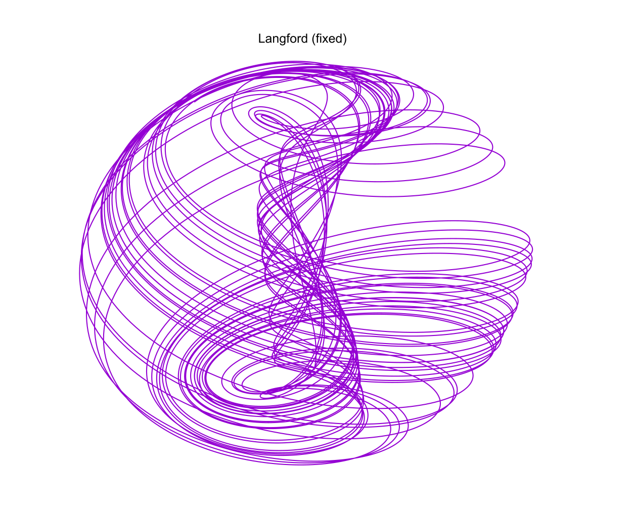
y_iv = [0.1_rk, 0.0_rk, 0.0_rk]
call steps_fixed_stab(status, istats, solution, eq, y_iv, param, a, b, c, t_delta_o=t_delta, max_pts_o=15000)
call print_solution(status, solution, filename_o="langford_fixed.csv", end_o=istats(1))

If we then load the data into Paraview, we get something like this:

We could also graph it with GNUplot:

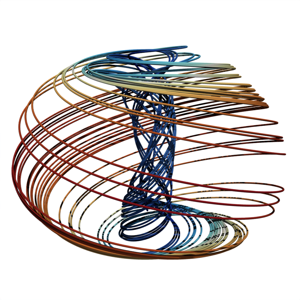
Just for fun, let's solve the IVP 20 times with diffrent initial values on a little circle on the central "stalk" structure. We can do that, in parallel, with this little bit of code:

!$OMP PARALLEL DO private(solution, status, istats, filename, i, y_iv)
do i=0, num_lines-1
   y_iv(1) = cos(i * 2 * pi / num_lines) * 0.15_rk + 0.2_rk
   y_iv(2) = sin(i * 2 * pi / num_lines) * 0.15_rk
   y_iv(3) = 0.05_rk
   call steps_fixed_stab(status, istats, solution, eq, y_iv, param, a, b, c, t_delta_o=t_delta, max_pts_o=350)
   write (filename, '("langford_",i2.2,".csv")') i
   call print_solution(status, solution, filename_o=trim(filename), end_o=istats(1), tag_o=i)
   print *, 'Line Complete: ', i
end do
!$OMP END PARALLEL DO

We can take the resulting 20 CSV files, load them up into Paraview, and animate the results:

2. Full Code Listing

2.1. Fortran Code

program langford
  use :: mrkiss_config,      only: rk, istats_size
  use :: mrkiss_solvers_nt,  only: steps_fixed_stab
  use :: mrkiss_utils,       only: print_solution
  use :: mrkiss_erk_kutta_4, only: a, b, c
  use :: omp_lib

  implicit none

  real(kind=rk),  parameter :: pi         = 4.0_rk * atan(1.0_rk)
  integer,        parameter :: num_lines  = 20
  integer,        parameter :: deq_dim    = 3
  integer,        parameter :: num_points = 100000
  real(kind=rk),  parameter :: param(6)   = [0.95_rk, 0.7_rk, 0.6_rk, 3.5_rk, 0.25_rk, 0.1_rk]
  real(kind=rk),  parameter :: t_delta    = 0.01_rk

  real(kind=rk)             :: solution(1+2*deq_dim, num_points), y_iv(deq_dim)
  integer                   :: status, istats(istats_size), i
  character(len=512)        :: filename

  y_iv = [0.1_rk, 0.0_rk, 0.0_rk]
  call steps_fixed_stab(status, istats, solution, eq, y_iv, param, a, b, c, t_delta_o=t_delta, max_pts_o=15000)
  call print_solution(status, solution, filename_o="langford_fixed.csv", end_o=istats(1))

  !$OMP PARALLEL DO private(solution, status, istats, filename, i, y_iv)
  do i=0, num_lines-1
     y_iv(1) = cos(i * 2 * pi / num_lines) * 0.15_rk + 0.2_rk
     y_iv(2) = sin(i * 2 * pi / num_lines) * 0.15_rk
     y_iv(3) = 0.05_rk
     call steps_fixed_stab(status, istats, solution, eq, y_iv, param, a, b, c, t_delta_o=t_delta, max_pts_o=350)
     write (filename, '("langford_",i2.2,".csv")') i
     call print_solution(status, solution, filename_o=trim(filename), end_o=istats(1), tag_o=i)
     print *, 'Line Complete: ', i
  end do
  !$OMP END PARALLEL DO

contains

  subroutine eq(status, dydt, y, param)
    integer,          intent(out) :: status
    real(kind=rk),    intent(out) :: dydt(:)
    real(kind=rk),    intent(in)  :: y(:), param(:)
    dydt = [(y(3) - param(2)) * y(1) - param(4) * y(2), 
            param(4)*y(1) + (y(3) - param(2))*y(2), 
            param(3) + param(1)*y(3) - (y(3)**3/3) - (y(1)**2+y(2)**2)*(1 + param(5)*y(3)) + param(6)*y(3)*y(1)**3]
    status = 0
  end subroutine eq

end program langford

2.2. GNUplot Code

The images were produced with GNUplot.

set encoding utf8
set termoption noenhanced
set datafile separator ','
set margins 0, 0, 0, 0
set view 50, 40, 1.3, 1.4
set xyplane at 0
unset border
unset ytics
unset ztics
unset xtics
set terminal svg
set pointsize 0.2

set title "Langford (fixed)"
set output "langford_fixed.svg"
splot 'langford_fixed.csv' using 3:4:5 with lines title ""

set title "Langford (fixed)"
set output "langford_multi.svg"
splot for [i=1:20] sprintf("langford_%02d.csv", i) using 4:5:6 with lines title ""

The multiple curve graph may be explored interactively with the following code.

set encoding utf8
set termoption noenhanced
set datafile separator ','
unset xlabel
unset ylabel
unset zlabel
unset grid
unset border
unset ytics
unset ztics
unset xtics
set view equal xyz
set view 160, 90

set title "Langford"
splot for [i=1:20] sprintf("langford_%02d.csv", i) using 4:5:6 with lines title ""

pause -1

The Langford Attractor A MRKISS Library Example Program

Table of Contents

1. Results

2. Full Code Listing

2.1. Fortran Code

2.2. GNUplot Code

The Langford Attractor
A MRKISS Library Example Program