MRKISS Library Example
Strange Attractors

Author:	Mitch Richling
Updated:	2025-07-26 14:43:32
Generated:	2025-07-26 14:43:35

1. Introduction
2. Curve Evoluation Animation
3. Sphere Sweeps
4. Limiting Step Length
5. Full Code Listing
- 5.1. Fortran Code
- 5.2. GNUplot Code

1. Introduction

The code for this example is found in examples/lornez.f90. Additionally the code may be found at the end of this document in the section Full Code Listing.

One strange thing when visualizing strange attracters is that we are frequently less concerned with the absolute accuracy of the solution curves than we are with the spacing of the solution points. This example uses the Lorenz attractor to explore some of the tools MRKISS provides for these kinds of problems.

2. Curve Evoluation Animation

For animations of the evolution of the curve, we normally use a fixed \(\Delta{t}\) because this preserves time in the animation so we can see the point tracing the curve speed up and slow down as the dirivative changes. We can produce such a solution with the steps_fixed_stab_*t() solvers. Here is an example of such a curve:

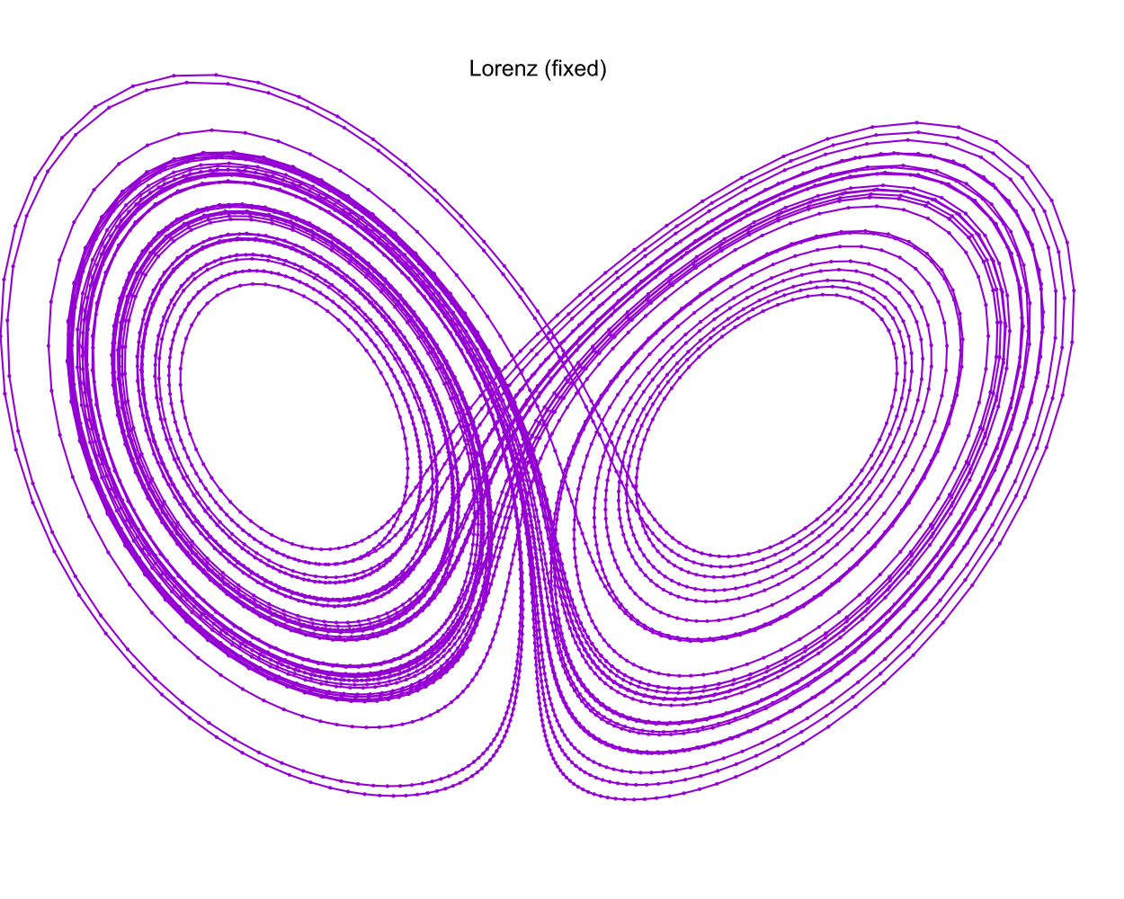
Notice the way some of the steps are much longer than others. This is especially apparnet in the upper right:

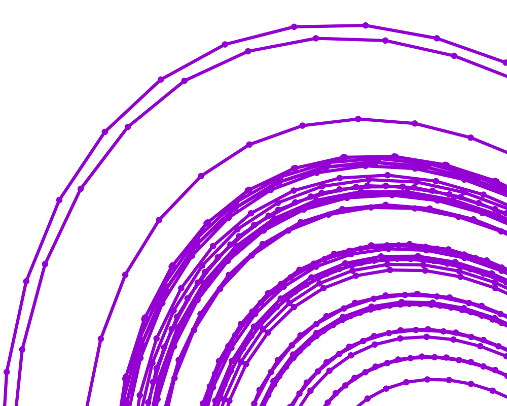
Many path animation tools have teh ablity to interpolate nitermediate points on peiceweise curves. SOme even have the ablty to use derviative information and do Hermite interpolation. Having a few longer steps when using such a tool is no issue. OTOH, when simply animating successve solution steps, large steps can make the animation jerkey. When this happens, if you still want to preserve time in the animation, the only real solution is to decrease the value used for \(\Delta{t}\).

THe solutions used in the images above were created by this snippit of examples/lornez.f90:

! BEGIN: lorenz_fixed
! This solution will have fixed t-delta, but no control over y-delta.
call system_clock(count_rate=c_rate)
call system_clock(c_beg)
call steps_fixed_stab_nt(status, istats, t_y_sol, eq, y_iv, param, a, b, c, t_delta_o=t_delta, t_max_o=t_max)
call system_clock(c_end)
print '(a,f10.3)', "fixed                      "
print '(a,i10)',   "                   Status: ", status
print '(a,f10.3)', "             Milliseconds: ", 1000*(c_end-c_beg)/DBLE(c_rate)
print '(a,i10)',   "          Solution Points: ", istats(1)
print '(a,i10)',   "   Regular one_step calls: ", istats(2)
print '(a,i10)',   "Adjustment one_step calls: ", istats(3)
call print_t_y_sol(status, t_y_sol, filename_o="lorenz_fixed.csv", end_o=istats(1), t_min_o=50.0_rk)
! END: lorenz_fixed

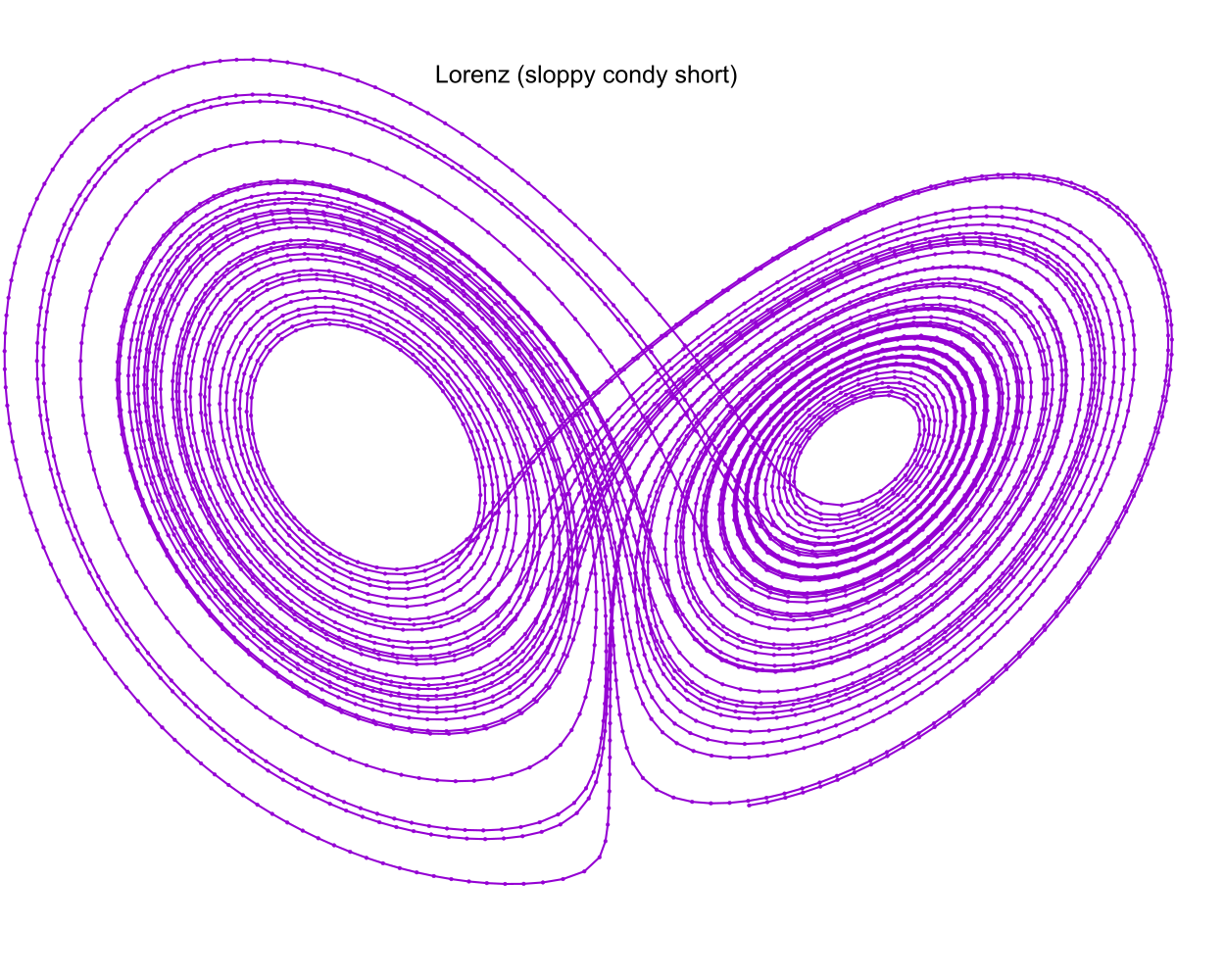
3. Sphere Sweeps

Ray tracing tools can render seines made up of spheres orders of magnitude faster than they can deal with things like triangle. Because of this fact it is common practice to represent curves in space as thousands, or millions, of spheres tightly packed along the curve – this is called a "sphere sweep". In order for this to work out the spheres need to be close together so that the angles of intersection are very small. Still we don't want too many spheres as every sphere adds time to the overall render. What we really want is to compute the optimal distance between the sphere centers, and then use this distance for all the spheres. That means we want steps of constant \(\mathbf{\Delta{y}}\).

Solutions with constant \(\mathbf{\Delta{y}}\) steps are also used for constant velocity animations of curve evolution. These can be interesting when done with groups of stream lines.

MRKISS provides two solvers for this situation:

steps_condy_stab_*t(): This solver uses considerable compute resources to insure that every step is the same length to a user provided tolerance. It requires the user provide minimum and maximum bounds for \(\Delta{t}\) which will bracket the correct value. The resulting curves are perfect for high quality sphere sweep renders.
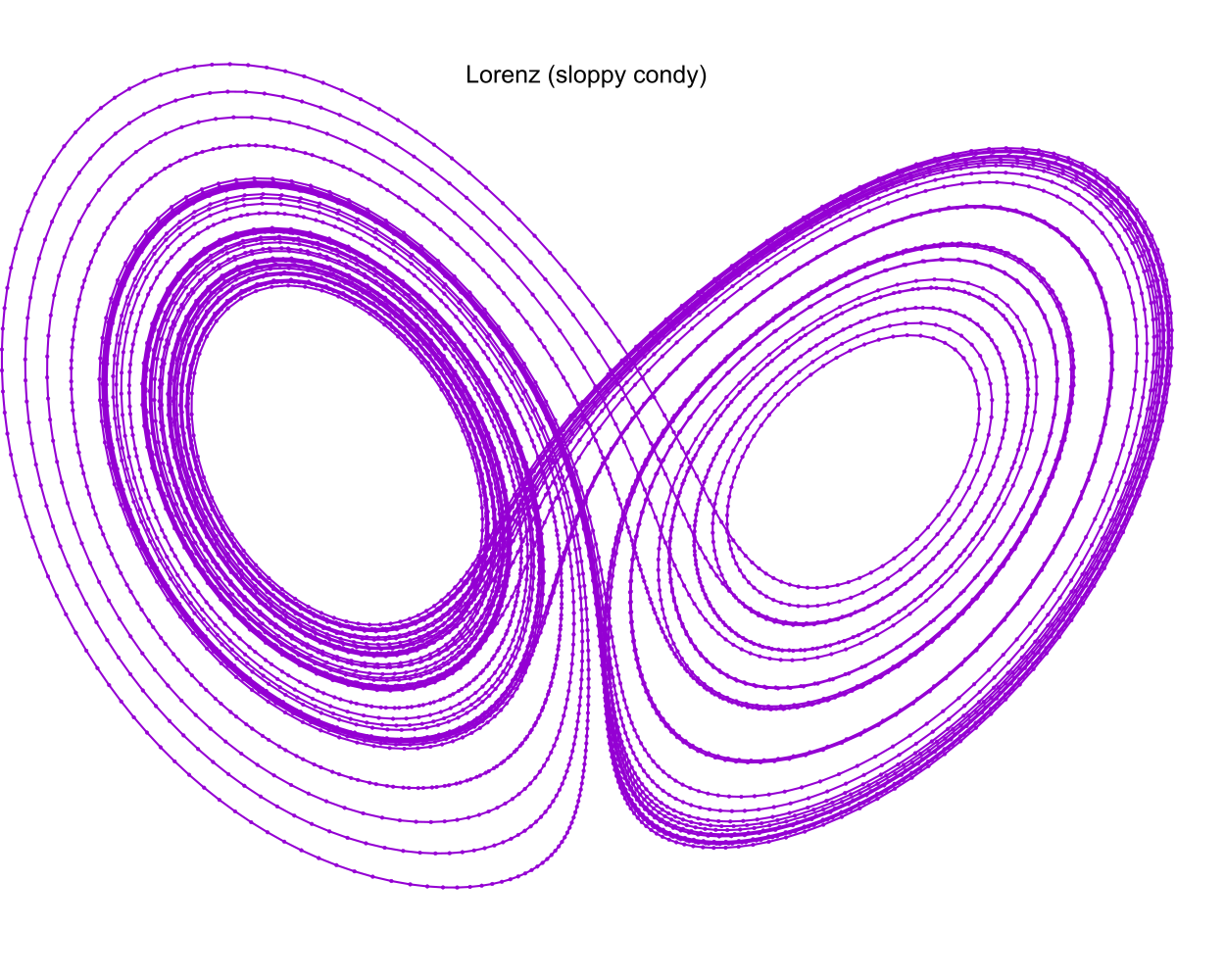
steps_sloppy_condy_stab_*t(): This solver only approximates optimal \(\Delta{t}\). In exchange for this inaccuracy, this routine is much faster than the previous option. The resulting solutions frequently good enough for a sphere sweep.

Here are some representative samples:

These images were created by the following snippet of examples/lornez.f90:

! BEGIN: lorenz_fixed-y
! This solution will have y-delta approximately capped to a maximum of 1.0 for all steps.
call system_clock(count_rate=c_rate)
call system_clock(c_beg)
call steps_sloppy_condy_stab_nt(status, istats, t_y_sol, eq, y_iv, param, a, b, c, 1.0_rk, t_delta, t_max_o=t_max)
call system_clock(c_end)
print '(a,f10.3)', "sloppy_condy               "
print '(a,i10)',   "                   Status: ", status
print '(a,f10.3)', "             Milliseconds: ", 1000*(c_end-c_beg)/DBLE(c_rate)
print '(a,i10)',   "          Solution Points: ", istats(1)
print '(a,i10)',   "   Regular one_step calls: ", istats(2)
print '(a,i10)',   "Adjustment one_step calls: ", istats(3)
call print_t_y_sol(status, t_y_sol, filename_o="lorenz_sloppy_condy.csv", end_o=istats(1), t_min_o=50.0_rk)

! This solution will have y-delta approximately equal to 1.0 for all steps.
call system_clock(count_rate=c_rate)
call system_clock(c_beg)
call steps_sloppy_condy_stab_nt(status, istats, t_y_sol, eq, y_iv, param, a, b, c, 1.0_rk, t_delta, t_max_o=t_max, &
                                adj_short_o=1)
call system_clock(c_end)
print '(a,f10.3)', "sloppy_condy short         "
print '(a,i10)',   "                   Status: ", status
print '(a,f10.3)', "             Milliseconds: ", 1000*(c_end-c_beg)/DBLE(c_rate)
print '(a,i10)',   "          Solution Points: ", istats(1)
print '(a,i10)',   "   Regular one_step calls: ", istats(2)
print '(a,i10)',   "Adjustment one_step calls: ", istats(3)
call print_t_y_sol(status, t_y_sol, filename_o="lorenz_sloppy_condy_short.csv", end_o=istats(1), t_min_o=50.0_rk)
! END: lorenz_fixed-y

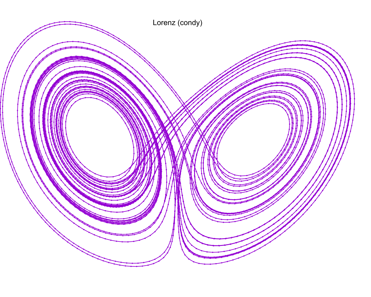
4. Limiting Step Length

When drawing line plots of curves we normally want them to be appear smooth which means we must avoid large values for \(\mathbf{\Delta{y}}\). For curve line drawing we normally are not terribly concerned with having a few short intervals because they don't have a huge impact on rendering speed.

When rendering curves as tubes most tools render a sphere at each point and a cylinder connecting the points. As with line drawings we want the curve to appear smooth, and so we wish to avoid large values for \(\mathbf{\Delta{y}}\). When rendering tubes we are more sensitive to excessive numbers of short intervals because every point impacts rendering speed. In addition, with some tools, very short intervals can introduce rendering glitches.

Of course we can use steps_condy_stab_*t() and steps_sloppy_condy_stab_*t(..., adj_short_o=1) as we did in the previous section; however, steps_sloppy_condy_stab_*t() without the adj_short_o=1 argument that may be more useful. Without this option only steps longer than the target are adjusted.

Here is the result:

The solution used in the image above was created by this snippet of examples/lornez.f90:

! BEGIN: lorenz_clip-y
! This solution will have y-delta equal to 1.0 for all steps.
call system_clock(count_rate=c_rate)
call system_clock(c_beg)
call steps_condy_stab_nt(status, istats, t_y_sol, eq, y_iv, param, a, b, c, 1.0_rk, t_delta*7, t_max_o=t_max)
call system_clock(c_end)
print '(a,f10.3)', "condy                      "
print '(a,i10)',   "                   Status: ", status
print '(a,f10.3)', "             Milliseconds: ", 1000*(c_end-c_beg)/DBLE(c_rate)
print '(a,i10)',   "          Solution Points: ", istats(1)
print '(a,i10)',   "   Regular one_step calls: ", istats(2)
print '(a,i10)',   "Adjustment one_step calls: ", istats(3)
call print_t_y_sol(status, t_y_sol, filename_o="lorenz_condy.csv", end_o=istats(1), t_min_o=50.0_rk)
! END: lorenz_clip-y

5. Full Code Listing

5.1. Fortran Code

!-------------------------------------------------------------------------------------------------
program lorenz
  use, intrinsic :: iso_fortran_env,    only: output_unit, error_unit
  use            :: mrkiss_config,      only: rk, ik, t_delta_tiny
  use            :: mrkiss_solvers_nt,  only: steps_fixed_stab_nt, steps_sloppy_condy_stab_nt, steps_condy_stab_nt
  use            :: mrkiss_utils,       only: print_t_y_sol
  use            :: mrkiss_erk_kutta_4, only: a, b, c

  implicit none

  integer,        parameter :: deq_dim       = 3
  integer,        parameter :: num_points    = 100000
  real(kind=rk),  parameter :: y_iv(deq_dim) = [1.0_rk, 0.0_rk, 0.0_rk]
  real(kind=rk),  parameter :: param(3)      = [10.0_rk, 28.0_rk, 8.0_rk/3.0_rk]
  real(kind=rk),  parameter :: t_delta       = 0.01_rk
  real(kind=rk),  parameter :: t_max         = 100.0_rk

  real(kind=rk)             :: t_y_sol(1+deq_dim, num_points)
  integer(kind=ik)          :: status, istats(16)
  integer                   :: c_beg, c_end, c_rate

  ! BEGIN: lorenz_fixed
  ! This solution will have fixed t-delta, but no control over y-delta.
  call system_clock(count_rate=c_rate)
  call system_clock(c_beg)
  call steps_fixed_stab_nt(status, istats, t_y_sol, eq, y_iv, param, a, b, c, t_delta_o=t_delta, t_max_o=t_max)
  call system_clock(c_end)
  print '(a,f10.3)', "fixed                      "
  print '(a,i10)',   "                   Status: ", status
  print '(a,f10.3)', "             Milliseconds: ", 1000*(c_end-c_beg)/DBLE(c_rate)
  print '(a,i10)',   "          Solution Points: ", istats(1)
  print '(a,i10)',   "   Regular one_step calls: ", istats(2)
  print '(a,i10)',   "Adjustment one_step calls: ", istats(3)
  call print_t_y_sol(status, t_y_sol, filename_o="lorenz_fixed.csv", end_o=istats(1), t_min_o=50.0_rk)
  ! END: lorenz_fixed

  ! BEGIN: lorenz_fixed-y
  ! This solution will have y-delta approximately capped to a maximum of 1.0 for all steps.
  call system_clock(count_rate=c_rate)
  call system_clock(c_beg)
  call steps_sloppy_condy_stab_nt(status, istats, t_y_sol, eq, y_iv, param, a, b, c, 1.0_rk, t_delta, t_max_o=t_max)
  call system_clock(c_end)
  print '(a,f10.3)', "sloppy_condy               "
  print '(a,i10)',   "                   Status: ", status
  print '(a,f10.3)', "             Milliseconds: ", 1000*(c_end-c_beg)/DBLE(c_rate)
  print '(a,i10)',   "          Solution Points: ", istats(1)
  print '(a,i10)',   "   Regular one_step calls: ", istats(2)
  print '(a,i10)',   "Adjustment one_step calls: ", istats(3)
  call print_t_y_sol(status, t_y_sol, filename_o="lorenz_sloppy_condy.csv", end_o=istats(1), t_min_o=50.0_rk)

  ! This solution will have y-delta approximately equal to 1.0 for all steps.
  call system_clock(count_rate=c_rate)
  call system_clock(c_beg)
  call steps_sloppy_condy_stab_nt(status, istats, t_y_sol, eq, y_iv, param, a, b, c, 1.0_rk, t_delta, t_max_o=t_max, &
                                  adj_short_o=1)
  call system_clock(c_end)
  print '(a,f10.3)', "sloppy_condy short         "
  print '(a,i10)',   "                   Status: ", status
  print '(a,f10.3)', "             Milliseconds: ", 1000*(c_end-c_beg)/DBLE(c_rate)
  print '(a,i10)',   "          Solution Points: ", istats(1)
  print '(a,i10)',   "   Regular one_step calls: ", istats(2)
  print '(a,i10)',   "Adjustment one_step calls: ", istats(3)
  call print_t_y_sol(status, t_y_sol, filename_o="lorenz_sloppy_condy_short.csv", end_o=istats(1), t_min_o=50.0_rk)
  ! END: lorenz_fixed-y

  ! BEGIN: lorenz_clip-y
  ! This solution will have y-delta equal to 1.0 for all steps.
  call system_clock(count_rate=c_rate)
  call system_clock(c_beg)
  call steps_condy_stab_nt(status, istats, t_y_sol, eq, y_iv, param, a, b, c, 1.0_rk, t_delta*7, t_max_o=t_max)
  call system_clock(c_end)
  print '(a,f10.3)', "condy                      "
  print '(a,i10)',   "                   Status: ", status
  print '(a,f10.3)', "             Milliseconds: ", 1000*(c_end-c_beg)/DBLE(c_rate)
  print '(a,i10)',   "          Solution Points: ", istats(1)
  print '(a,i10)',   "   Regular one_step calls: ", istats(2)
  print '(a,i10)',   "Adjustment one_step calls: ", istats(3)
  call print_t_y_sol(status, t_y_sol, filename_o="lorenz_condy.csv", end_o=istats(1), t_min_o=50.0_rk)
  ! END: lorenz_clip-y

contains

  subroutine eq(status, dydt, y, param)
    integer(kind=ik), intent(out) :: status
    real(kind=rk),    intent(out) :: dydt(:)
    real(kind=rk),    intent(in)  :: y(:)
    real(kind=rk),    intent(in)  :: param(:)
    dydt(1) = param(1)*(y(2)-y(1))       ! a(y-x)
    dydt(2) = y(1)*(param(2)-y(3))-y(2)  ! x(b-z)-y
    dydt(3) = y(1)*y(2)-param(3)*y(3)    ! xy-cy
    status = 0
  end subroutine eq

end program

5.2. GNUplot Code

The images were produced with R.

#------------------------------------------------------------------------------------------------------------------------------
set encoding utf8
set termoption noenhanced
set datafile separator ','
# set xlabel "x"
# set ylabel "y"
# set zlabel "z"
#set grid
set margins 0, 0, 0, 0
set view 70, 40, 1.3, 1.4
set xyplane at 0
unset border
unset ytics
unset ztics
unset xtics
set terminal svg
set pointsize 0.2

set title "Lorenz (fixed)"
set output "lorenz_fixed.svg"
splot 'lorenz_fixed.csv' using 3:4:5 with linespoints pt 7 title ""

set title "Lorenz (sloppy condy)"
set terminal svg
set output "lorenz_sloppy_condy.svg"
splot 'lorenz_sloppy_condy.csv' using 3:4:5 with linespoints pt 7 title ""

set title "Lorenz (sloppy condy short)"
set terminal svg
set output "lorenz_sloppy_condy_short.svg"
splot 'lorenz_sloppy_condy_short.csv' using 3:4:5 with linespoints pt 7 title ""

set title "Lorenz (condy)"
set terminal svg
set output "lorenz_condy.svg"
splot 'lorenz_condy.csv' using 3:4:5 with linespoints pt 7 title ""

MRKISS Library Example Strange Attractors

Table of Contents