A Three Body Problem
A MRKISS Library Example Program

Author:	Mitch Richling
Updated:	2025-09-10 16:56:01
Generated:	2025-09-10 16:56:02

1. Introduction
2. Classical Solution
3. Interpolation
4. Fixed Steps & Method Order
5. Adaptive Solution With More Steps For A Nice Plot
6. Truly Fixed Steps in y-space
7. Knowing When To Stop
8. Satellite & Moon Orbit Intersection
9. Full Code Listing
- 9.1. Fortran Code
- 9.2. R Code

1. Introduction

The code for this example is found in MRKISS/examples/three_body.f90. Additionally the code may be found at the end of this document in the section Full Code Listing.

This example makes several MRKISS high level solver calls each illustrating a different feature or technique. In the sections that follow we examine each of those calls in detail.

This is one of my favorite IVP example problems.

This is a dimensionless, restricted three gravitational body problem. The Earth is stationary at the origin. The Moon orbits the Earth at a radius of \(1\) and is at \((1,0)\) at \(t=0\). The Moon to Earth mass ratio is \(\frac{100}{8145}\). We wish to model the movement of a small satellite with negligible mass. The position, \((x_1,x_2)\), and velocity, \((v_1,v_2)\), of this satellite are governed by the following differential equation:

\[\begin{align*} \frac{\mathrm{d}v_1}{\mathrm{d}t} & = v_1 \\ \frac{\mathrm{d}v_2}{\mathrm{d}t} & = v_2 \\ \frac{\mathrm{d}x_1}{\mathrm{d}t} & = 2 v_2 + x_1 - \frac{\mu (x_1 + \mu -1)}{D_1} - \frac{(1 - \mu) (x_1 + \mu)}{D_2} \\ \frac{\mathrm{d}x_2}{\mathrm{d}t} & = -2 v_1 + x_2 - \frac{\mu x_2}{D_1} - \frac{(1 - \mu) x_2}{D_2} \end{align*}\]

Where \(D_1\) and \(D_2\) are defined as:

\[\begin{align*} D_1 & = \sqrt{\left(x_2^2 + (x_1 + \mu - 1)^2\right)^3} \\ D_2 & = \sqrt{\left(x_2^2 + (x_1 + \mu)\right)^3} \end{align*}\]

We solve the equations with the following initial values:

\[\begin{align*} (x_1,x_2) &= \left(\frac{497}{500}, 0\right) \\ (v_1,v_2) & = (0, -2.0015851063790825224) \end{align*}\]

Under these conditions the satellite will return to it's initial position after completing a three lobed orbit at \(t=17.06521656015796\).

Another interesting set of initial conditions leads to a five lobe orbit at \(t=19.14045706162071\):

\[\begin{align*} (x_1,x_2) &= \left(0.87978, 0\right) \\ (v_1,v_2) & = (0, -0.3797) \end{align*}\]

References:

Arenstorf (1963); Periodic Solutions of the Restricted Three Body Problem Representing Analytic Continuations of Keplerian Elliptic Motions; American J. of Math. 85 (1); p27-35;
Butcher (2008); Numerical Methods for Ordinary Differential Equations. 2ed; p29-30;
Butcher (2016); Numerical Methods for Ordinary Differential Equations. 3ed; p28-31;
Hairer, Norsett & Wanner (2009). Solving Ordinary Differential Equations. I: Nonstiff Problems. p129-130;

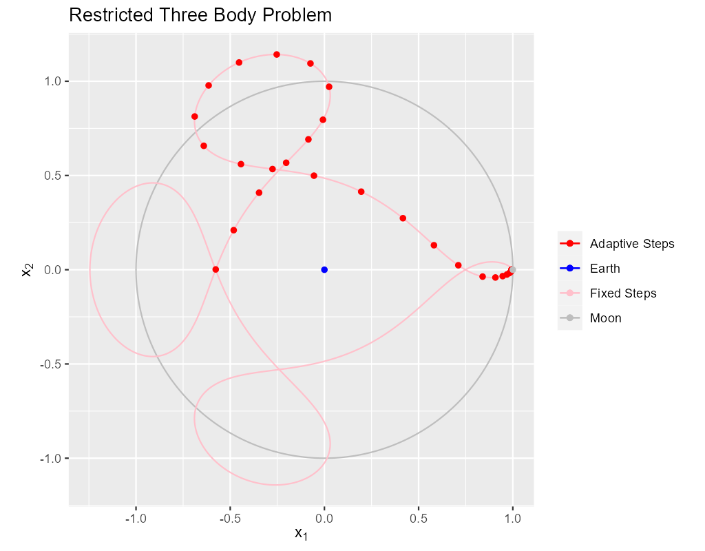
2. Classical Solution

In this section we produce the classical image of the solution.

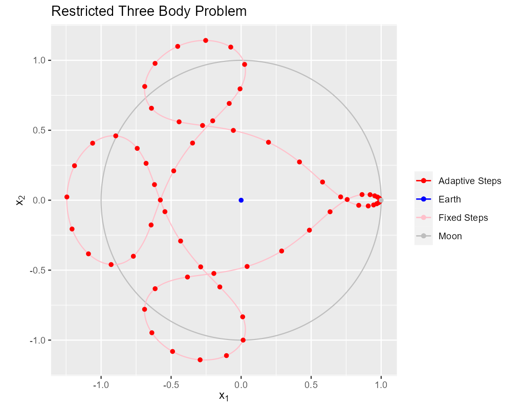
The solid pink curve is generated from 4000 points on the orbit generated with a fixed step size solver. This is quite expensive computationally taking about 16 milliseconds on my computer. Still, it produces a very nice curve.

call fixed_t_steps(status, istats1, sol1, eq, t_iv, y_iv, param, a, b, c, t_end_o=t_end)
print '(a)', status_to_message(status)
call print_istats(status, istats1)
call print_solution(status, sol1, filename_o="tree_body_fixed_t_steps.csv", end_o=istats1(1))

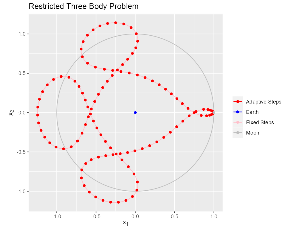
The red dots on the solid pink curve are solution points generated using a classical, adaptive Runge-Kutta scheme.

The algorithms involved in the adaptive solution are far more complex than in the fixed step solution above. Yet the solver calls in these two code snippets are remarkably similar. IMO, the real value in an adaptive solver is the reduction in computational needs by making the step sizes as large as possible without sacrificing accuracy. As you can see the step size is much smaller near the singularities. The fixed run above takes 16 milliseconds while the adaptive run takes less than one millisecond.

More sophisticated libraries offer the ability to interpolate between solution points at pretty low cost while maintaining the accuracy of the overall method. For generative art and visualization we can use Hermite interpolation at an even lower cost. Normally interpolation is not performed in the ODE solver, but directly by a visualization software platform – we simply provide the points and derivatives.

call adaptive_steps(status, istats1, sol1, eq, t_iv, y_iv, param, a, b, c, p, &
                         t_delta_max_o=t_delta*100, t_delta_ini_o=t_delta*20, error_tol_abs_o=[1.0e-9_rk], &
                         error_tol_rel_o=[1.0e-6_rk], t_max_o=t_end);
print '(a)', status_to_message(status)
call print_istats(status, istats1)
call print_solution(status, sol1, filename_o="three_body_adaptive_steps-std.csv", end_o=istats1(1))

3. Interpolation

Most visualization tools directly support Hermite spline interpolation between points, and will happily use use the derivative information in the solution to connect the widely separated red dots in the adaptive solution with smooth curves. So it is rare that we wish to do interpolation simply to connect dots. More common is the need to "line up" two solutions on the same \(t\) values for some other reason. The most common use case is Hermite interpolation:

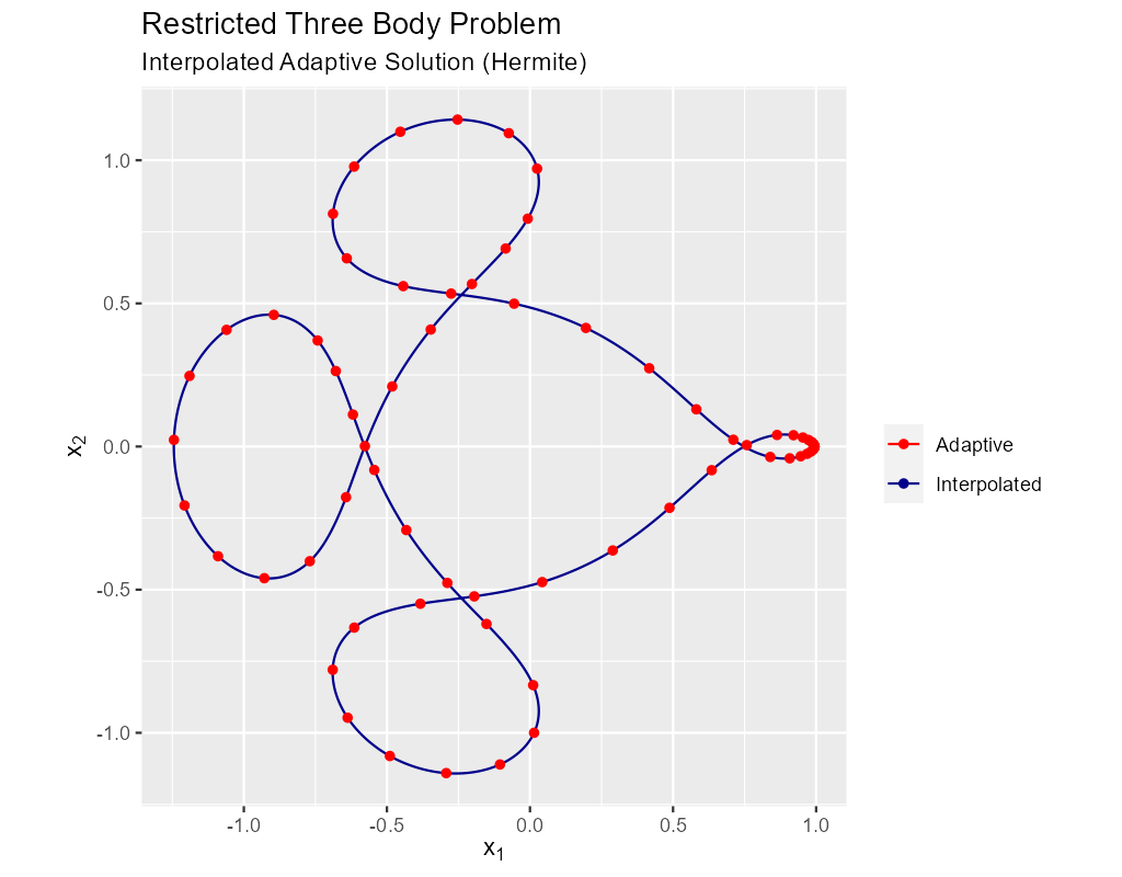
The data for the image above was produced by this code:

call seq(status, sol2(1,:), from_o=0.0_rk, to_o=t_end);                                     ! Create new t values
print '(a)', status_to_message(status)
call interpolate_solution(status, istats2, sol2, sol1, eq, param, num_src_pts_o=istats1(1)) ! Preform the interpolation
call print_solution(status, sol2, filename_o="three_body_steps_adapt_std_interpolated.csv")

Less common is linear interpolation:

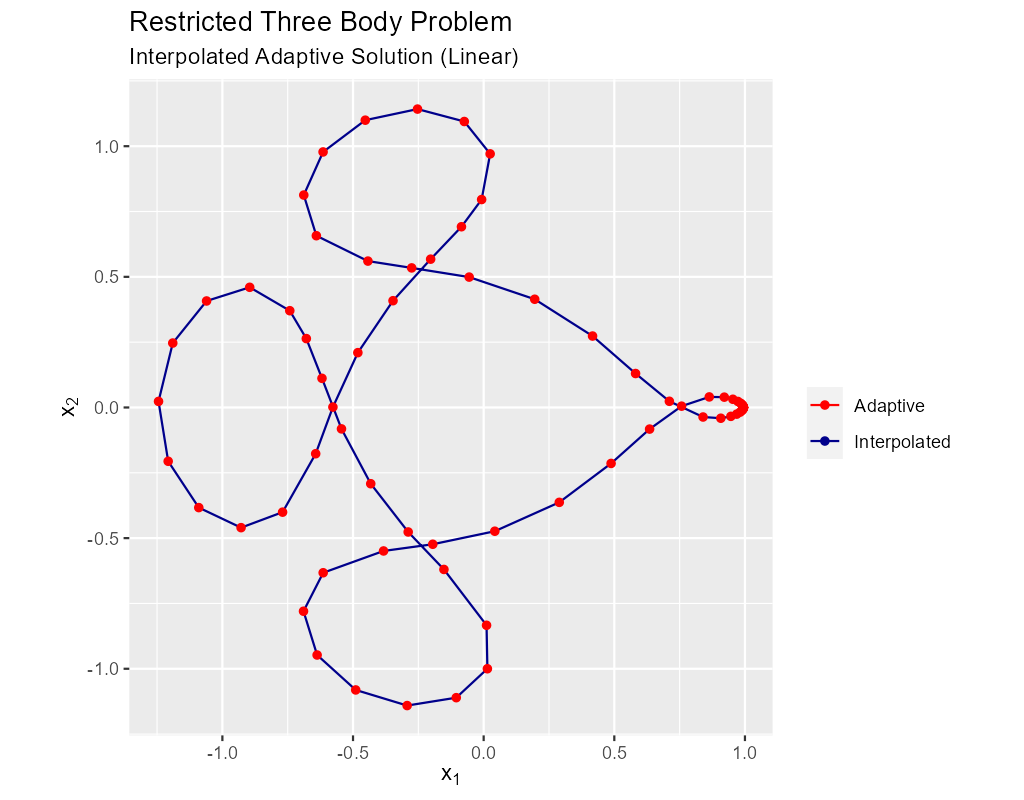
The data for the image above was produced by this code:

call seq(status, sol2(1,:), from_o=0.0_rk, to_o=t_end);
call interpolate_solution(status, istats2, sol2, sol1, eq, param, num_src_pts_o=istats1(1), linear_interp_o=.true.)
print '(a)', status_to_message(status)
call print_solution(status, sol2, filename_o="three_body_steps_adapt_std_interpolated_lin.csv")

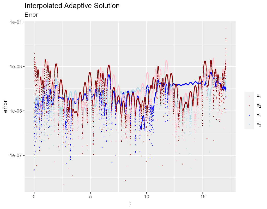
Note that Hermite interpolation provides an O(3) solution to the IVP, but that may still be inappropriate if high accuracy solutions are required. Here we can see the errors in Hermite interpolation used above:

4. Fixed Steps & Method Order

The pink curve in our first image was the result of 4000 fixed steps with a 9th order Runge-Kutta method. Why did we pick a 9th order solver? Because it allowed us to use a step size small enough to be ascetically pleasing but large enough to not produce too many points for our simple plotting program.

From the perspective of generative art and visualization, fixed time step solutions are important because they preserve "time" in animations. We can achieve fixed steps via interpolation; however, it is frequently more convenient to simply use a fixed step size solver. Method order for generative art and visualization is often thought of as a tool to allow for aesthetic step sizes instead of a way to achieve a solution accuracy requirement.

In the following image we see the unsatisfactory result of using a 5th order solver with the same step size:

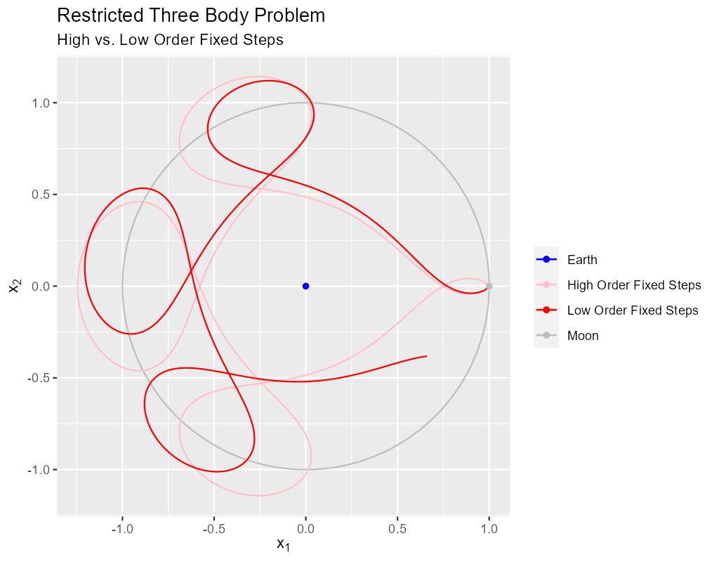
The code for the above solution is identical except for a change in Runge-Kutta method arguments:

call fixed_t_steps(status, istats1, sol1, eq, t_iv, y_iv, param, dpa, dpb, dpc, t_end_o=t_end)
print '(a)', status_to_message(status)
call print_istats(status, istats1)
call print_solution(status, sol1, filename_o="fixed_t_steps-dp.csv", end_o=istats1(1))

5. Adaptive Solution With More Steps For A Nice Plot

If we wanted more points in the adaptive solution we could use t_delta_max_o. This will get us more points, but it's not necessarily what we want for a nice graph. What we really want for a nice graph is a fixed maximum distance between plotted points which a fixed \(\Delta{t}\) will not necessarily deliver. That said we still want the adaptive algorithm to produce points closer together when accuracy requires it. One way to achieve that is with the step processing capability of adaptive_steps() via the stepp_o argument. Only the first two components of the solution are plotted (the position of the satellite). What we want the stepp_o subroutine to do is shrink \(\Delta{t}\) if the distance between the first two components of the solution are too far away from the first two points of the previous solution. The following subroutine will do the trick:

! Example subroutine to adjust t_delta in an attempt to keep y_delta under a maximum value.
! It is sloppy because we assume t_delta is linearly proportional to y_delta_len
subroutine sp_sloppy_y_delta_len_max(status, end_run, sdf_flags, new_t_delta, pnt_idx, solution, t_delta, y_delta)
  integer,          intent(out) :: status, end_run
  real(kind=rk),    intent(out) :: new_t_delta
  integer,          intent(out) :: sdf_flags
  integer,          intent(in)  :: pnt_idx
  real(kind=rk),    intent(in)  :: solution(:,:), t_delta, y_delta(:)
  real(kind=rk),      parameter :: y_delta_len_max = 0.1_rk
  integer,            parameter :: y_delta_len_idxs(2) = [1, 2]
  real(kind=rk)                 :: y_delta_len
  status    = 0
  end_run   = 0
  sdf_flags = 0
  y_delta_len = norm2(y_delta(y_delta_len_idxs))
  if ( y_delta_len > y_delta_len_max) then
     new_t_delta = t_delta * y_delta_len_max / y_delta_len
  else
     new_t_delta = -1.0_rk
  end if
end subroutine sp_sloppy_y_delta_len_max

This isn't a perfect solution as we make the assumption that the length of the difference in \(\mathbf{y}\mathrm{-space}\) is proportional to \(\Delta{t}\), but it works pretty well in practice. A more robust solution can be achieved by adding an sdf_o function and isolating a \(\Delta{t}\) that produces a precisely separated solution. We touch on this topic later when we consider the fixed_y_steps() solvers.

We "wire up" the above subroutine into adaptive_steps() via the stepp_o argument.

call adaptive_steps(status, istats1, sol1, eq, t_iv, y_iv, param, a, b, c, p, &
                         t_delta_max_o=t_delta*100, t_delta_ini_o=t_delta*20, error_tol_abs_o=[1.0e-9_rk], &
                         error_tol_rel_o=[1.0e-6_rk], t_max_o=t_end, t_end_o=t_end, &
                         stepp_o=sp_sloppy_y_delta_len_max);
print '(a)', status_to_message(status)
call print_istats(status, istats1)
call print_solution(status, sol1, filename_o="three_body_adaptive_steps-fix-delta-steps.csv", end_o=istats1(1))

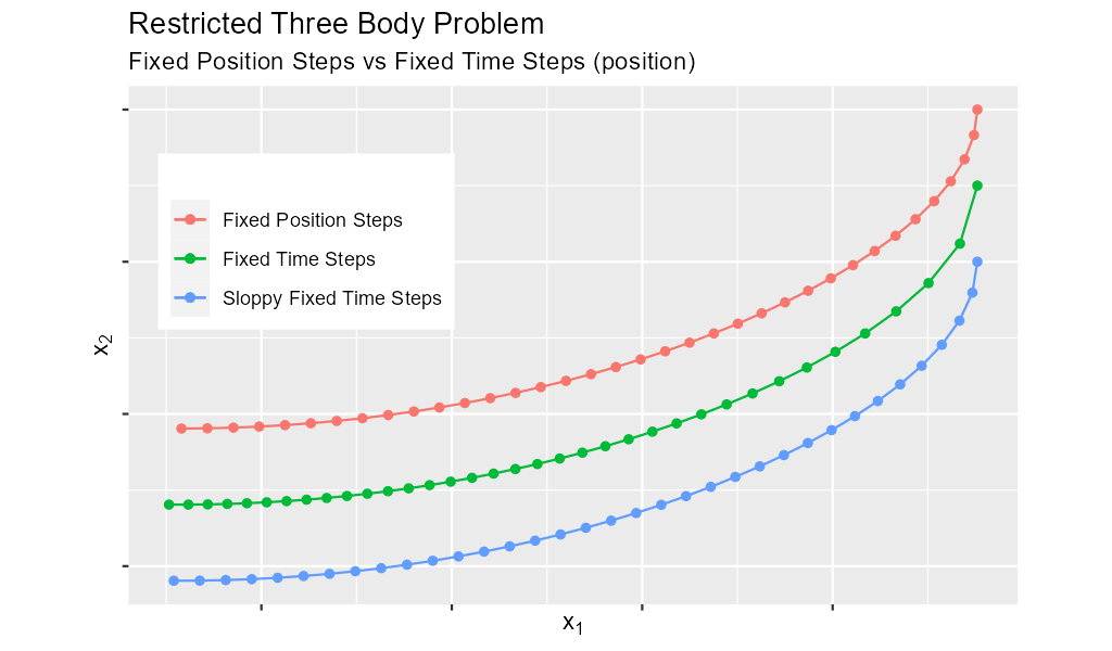
6. Truly Fixed Steps in y-space

We can achieve truly fixed step sizes in \(\mathbf{y}\mathrm{-space}\) with the fixed_y_steps() solvers. In the image below we see the difference between fixed steps in \(t\mathrm{-space}\) vs \(\mathbf{y}\mathrm{-space}\) – remember we are only using the position components of the \(\mathbf{y}\) vector (the first two components) and not the velocity components (the last two components).

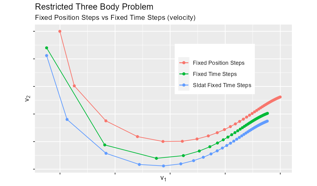
Below are the velocity components plotted in the same manner as the position components. Notice the wildly differing distances between the solution points.

In the code below we set y_delta_len_idxs_o to [1, 2] in order to have fixed_y_steps() only use the first two components of the solution vector in it's length computation. This will produce steps that are 0.0034 long with an accuracy of 1.0e-5.

call fixed_y_steps(status, istats1, sol1, eq, t_iv, y_iv, param, a, b, c, 0.0034_rk, .01_rk, &
                         y_delta_len_idxs_o=[1,2], y_sol_len_max_o=path_length, y_delta_len_tol_o=1.0e-5_rk)
print '(a)', status_to_message(status)
call print_istats(status, istats1)

call print_solution(status, sol1, filename_o="three_body_fixed_y_steps.csv", end_o=istats1(1))

We can also achieve a sloppy constant length \(\mathbf{y}\mathrm{-space}\) much like we did previously with adaptive_steps() but with sloppy_fixed_y_steps().

call sloppy_fixed_y_steps(status, istats1, sol1, eq, t_iv, y_iv, param, a, b, c, 0.0034_rk, .01_rk, &
                                y_delta_len_idxs_o=[1,2], y_sol_len_max_o=path_length)
print '(a)', status_to_message(status)
call print_istats(status, istats1)
call print_solution(status, sol1, filename_o="sloppy_fixed_y_steps.csv", end_o=istats1(1))

7. Knowing When To Stop

Sometimes you don't know beforehand when you want the solver to stop. This is another place where stepp_o can help. For this example we simply tell the solver to stop when we get past a particular value of \(t\). Of course we could have done this with the t_max_o argument. The next section will explore a more realistic example.

The idea is to use a subroutine for stepp_o that will tell adaptive_steps() to quit when we hit a maximum value for \(t\). The following code will do the trick:

! Example subroutine replicating the functionality of t_max_o in adaptive_steps().
subroutine sp_max_t(status, end_run, sdf_flags, new_t_delta, pnt_idx, solution, t_delta, y_delta)
  integer,          intent(out) :: status
  integer,          intent(out) :: end_run
  real(kind=rk),    intent(out) :: new_t_delta
  integer,          intent(out) :: sdf_flags
  integer,          intent(in)  :: pnt_idx
  real(kind=rk),    intent(in)  :: solution(:,:), t_delta, y_delta(:)
  real(kind=rk),    parameter   :: t_max = 6.2_rk
  status    = 0
  sdf_flags = 0
  new_t_delta = -1.0_rk
  if ( solution(1, pnt_idx-1) + t_delta > t_max) then
     end_run = 1
  else
     end_run = 0
  end if
end subroutine sp_max_t

We wire up this subroutine to adaptive_steps() via the stepp_o argument like so:

call adaptive_steps(status, istats1, sol1, eq, t_iv, y_iv, param, a, b, c, p, &
                         t_delta_max_o=t_delta*100, t_delta_ini_o=t_delta*20, error_tol_abs_o=[1.0e-9_rk], &
                         error_tol_rel_o=[1.0e-6_rk], t_max_o=t_end, t_end_o=t_end, &
                         stepp_o=sp_max_t);
print '(a)', status_to_message(status)
call print_istats(status, istats1)
call print_solution(status, sol1, filename_o="three_body_adaptive_steps-pho-t-max.csv", end_o=istats1(1))

8. Satellite & Moon Orbit Intersection

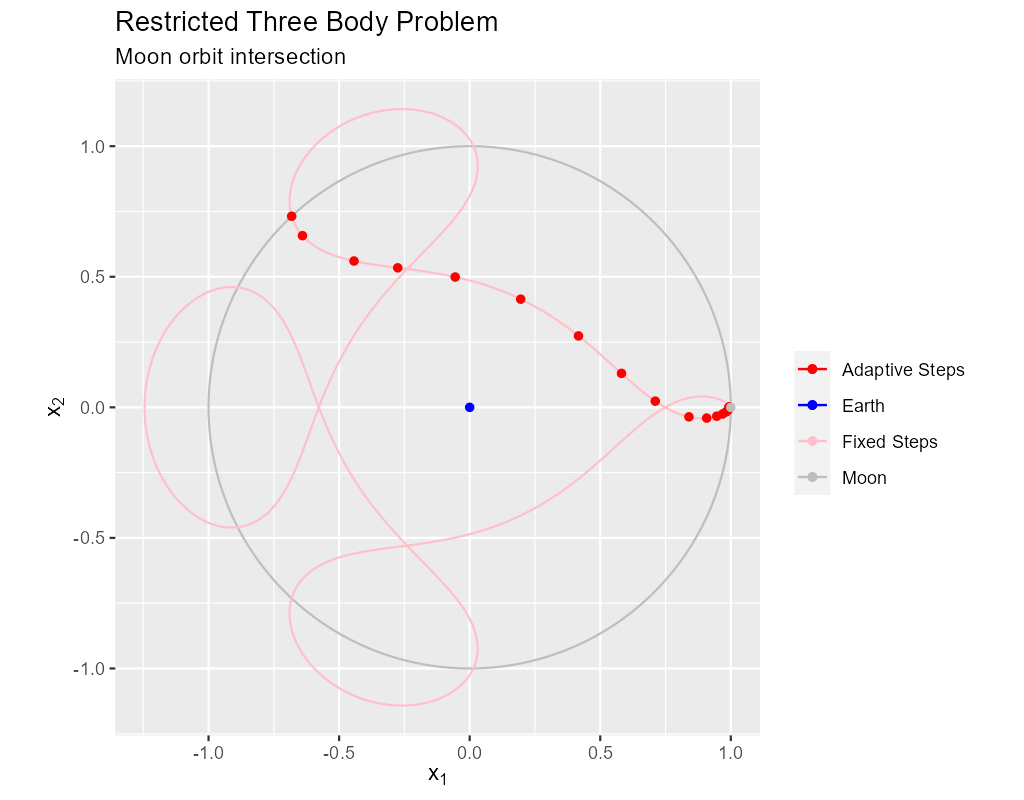
In the image above note the last adaptive point is precisely on the intersection of the satellite and moon orbit. We could easily stop with a stepp_o routine after we cross the moon orbit – much like we did in the previous section. If we did that we would have a final solution segment that straddled the orbit, but it is unlikely that the final end point would be precisely on the orbit. What we need here is a way to find a \(\Delta{t}\) for our last interval that leads to a solution that precisely hits the moon's orbit. We can do that by adding and sdf_o subroutine and having our stepp_o subroutine tell adaptive_steps() when to use it.

Lets take a look at the stepp_o subroutine first. This routine first checks to see if the solution point is on the moon's orbit, and tells adaptive_steps() to quit if it is. This is very unlikely to happen, but we check anyhow. Next it checks to see if the solution segment straddles the moons orbit – i.e. if the previous solution was on one side of the orbit while the current on is on the other. If this occurs the stepp_o tells adaptive_steps() two things: 1) Solve for the final \(\Delta{t}\) with sdf_o, and 2) quit after this solution.

! Example subroutine to find the first intersection of the satellite path and the moon's orbit.  It works 
! in conjunction with sdf_cross_moon().
subroutine sp_cross_moon(status, end_run, sdf_flags, new_t_delta, pnt_idx, solution, t_delta, y_delta)
  integer,          intent(out) :: status, end_run
  real(kind=rk),    intent(out) :: new_t_delta
  integer,          intent(out) :: sdf_flags
  integer,          intent(in)  :: pnt_idx
  real(kind=rk),    intent(in)  :: solution(:,:), t_delta, y_delta(:)
  real(kind=rk),    parameter   :: eps = 0.0001_rk
  real(kind=rk)                 :: lp_d, cp_d    
  status      = 0
  sdf_flags   = 0
  end_run     = 0
  new_t_delta = -1.0_rk
  if (solution(1, pnt_idx-1) > 0.2_rk) then
     cp_d = norm2(solution(2:3, pnt_idx-1)+y_delta(1:2))
     if ( abs(cp_d-1.0_rk)  < eps) then
        end_run   = 1
     else
        lp_d = norm2(solution(2:3, pnt_idx-1))
        if ((min(lp_d, cp_d) < 1.0_rk) .and. (max(lp_d, cp_d) > 1.0_rk)) then
           sdf_flags = 1
           end_run   = 1
        end if
     end if
  end if
end subroutine sp_cross_moon

The magical SDF function is pretty simple in this case. The moon's orbit in this scaled problem is the unit circle, so we just have to subtract the norm of the solution's position from 1!

! Example SDF subroutine to isolate a point on a solution segment that crosses the unit circle.
subroutine sdf_cross_moon(status, dist, sdf_flags, t, y)
  use mrkiss_config, only: rk
  implicit none
  integer,          intent(out) :: status
  real(kind=rk),    intent(out) :: dist
  integer,          intent(in)  :: sdf_flags
  real(kind=rk),    intent(in)  :: t, y(:)
  status = 0
  dist = 1.0_rk - norm2(y(1:2))
end subroutine sdf_cross_moon

As usual we wire these two functions up to adaptive_steps() via the stepp_o and sdf_o arguments.

call adaptive_steps(status, istats1, sol1, eq, t_iv, y_iv, param, a, b, c, p, &
                         t_delta_max_o=t_delta*100, t_delta_ini_o=t_delta*20, error_tol_abs_o=[1.0e-9_rk], &
                         error_tol_rel_o=[1.0e-6_rk], t_max_o=t_end, t_end_o=t_end, &
                         stepp_o=sp_cross_moon, sdf_o=sdf_cross_moon);
print '(a)', status_to_message(status)
call print_istats(status, istats1)
call print_solution(status, sol1, filename_o="three_body_adaptive_steps-isct.csv", end_o=istats1(1))

9. Full Code Listing

9.1. Fortran Code

program three_body
  use, intrinsic :: iso_fortran_env,                only: output_unit, error_unit
  use            :: mrkiss_config,                  only: rk, istats_size
  use            :: mrkiss_solvers_wt,              only: fixed_t_steps, fixed_y_steps, adaptive_steps, &
                                                          sloppy_fixed_y_steps, interpolate_solution
  use            :: mrkiss_utils,                   only: print_solution, seq, print_istats, status_to_message
  use            :: mrkiss_eerk_verner_9_8,         only: a, b, c, p
  use            :: mrkiss_eerk_dormand_prince_5_4, only: dpa=>a, dpb=>b, dpc=>c

  implicit none

  integer,          parameter :: deq_dim       = 4
  integer,          parameter :: num_points    = 4000
  real(kind=rk),    parameter :: t_iv          = 0.0_rk
  real(kind=rk),    parameter :: t_end         = 17.06521656015796_rk
  real(kind=rk),    parameter :: path_length   = 10.7068_rk 
  real(kind=rk),    parameter :: y_iv(deq_dim) = [0.994_rk, 0.0_rk, 0.0_rk, -2.0015851063790825224_rk]
  real(kind=rk),    parameter :: param(1)      = [1.0_rk / 81.45_rk]
  real(kind=rk),    parameter :: t_delta       = 17.06521656015796d0 / (num_points - 1 )

  real(kind=rk)               :: sol1(1+2*deq_dim, num_points), sol2(1+2*deq_dim, num_points)
  integer                     :: status, istats1(istats_size), istats2(istats_size)

  print '(a)', repeat('*', 120)
  print '(a)', "Fixed t_delta run V(9)"
  call fixed_t_steps(status, istats1, sol1, eq, t_iv, y_iv, param, a, b, c, t_end_o=t_end)
  print '(a)', status_to_message(status)
  call print_istats(status, istats1)
  call print_solution(status, sol1, filename_o="tree_body_fixed_t_steps.csv", end_o=istats1(1))

  print '(a)', repeat('*', 120)
  print '(a)', "Fixed t_delta run DP(5)"
  call fixed_t_steps(status, istats1, sol1, eq, t_iv, y_iv, param, dpa, dpb, dpc, t_end_o=t_end)
  print '(a)', status_to_message(status)
  call print_istats(status, istats1)
  call print_solution(status, sol1, filename_o="fixed_t_steps-dp.csv", end_o=istats1(1))

  print '(a)', repeat('*', 120)
  print '(a)', "Fixed y_delta run"
  call fixed_y_steps(status, istats1, sol1, eq, t_iv, y_iv, param, a, b, c, 0.0034_rk, .01_rk, &
                           y_delta_len_idxs_o=[1,2], y_sol_len_max_o=path_length, y_delta_len_tol_o=1.0e-5_rk)
  print '(a)', status_to_message(status)
  call print_istats(status, istats1)

  call print_solution(status, sol1, filename_o="three_body_fixed_y_steps.csv", end_o=istats1(1))

  print '(a)', repeat('*', 120)
  print '(a)', "Sloppy Fixed y_delta run"
  call sloppy_fixed_y_steps(status, istats1, sol1, eq, t_iv, y_iv, param, a, b, c, 0.0034_rk, .01_rk, &
                                  y_delta_len_idxs_o=[1,2], y_sol_len_max_o=path_length)
  print '(a)', status_to_message(status)
  call print_istats(status, istats1)
  call print_solution(status, sol1, filename_o="sloppy_fixed_y_steps.csv", end_o=istats1(1))

  print '(a)', repeat('*', 120)
  print '(a)', "Adaptive run"
  sol1 = 0
  call adaptive_steps(status, istats1, sol1, eq, t_iv, y_iv, param, a, b, c, p, &
                           t_delta_max_o=t_delta*100, t_delta_ini_o=t_delta*20, error_tol_abs_o=[1.0e-9_rk], &
                           error_tol_rel_o=[1.0e-6_rk], t_max_o=t_end);
  print '(a)', status_to_message(status)
  call print_istats(status, istats1)
  call print_solution(status, sol1, filename_o="three_body_adaptive_steps-std.csv", end_o=istats1(1))

  print '(a)', repeat('*', 120)
  print '(a)', "Hermite interpolation run"
  sol2 = 0
  call seq(status, sol2(1,:), from_o=0.0_rk, to_o=t_end);                                     ! Create new t values
  print '(a)', status_to_message(status)
  call interpolate_solution(status, istats2, sol2, sol1, eq, param, num_src_pts_o=istats1(1)) ! Preform the interpolation
  call print_solution(status, sol2, filename_o="three_body_steps_adapt_std_interpolated.csv")

  print '(a)', repeat('*', 120)
  print '(a)', "Linear interpolation run"
  sol2 = 0
  call seq(status, sol2(1,:), from_o=0.0_rk, to_o=t_end);
  call interpolate_solution(status, istats2, sol2, sol1, eq, param, num_src_pts_o=istats1(1), linear_interp_o=.true.)
  print '(a)', status_to_message(status)
  call print_solution(status, sol2, filename_o="three_body_steps_adapt_std_interpolated_lin.csv")

  print '(a)', repeat('*', 120)
  print '(a)', "Adaptive run w max y_delta length"
  call adaptive_steps(status, istats1, sol1, eq, t_iv, y_iv, param, a, b, c, p, &
                           t_delta_max_o=t_delta*100, t_delta_ini_o=t_delta*20, error_tol_abs_o=[1.0e-9_rk], &
                           error_tol_rel_o=[1.0e-6_rk], t_max_o=t_end, t_end_o=t_end, &
                           stepp_o=sp_sloppy_y_delta_len_max);
  print '(a)', status_to_message(status)
  call print_istats(status, istats1)
  call print_solution(status, sol1, filename_o="three_body_adaptive_steps-fix-delta-steps.csv", end_o=istats1(1))

  print '(a)', repeat('*', 120)
  print '(a)', "Adaptive run w max t"
  call adaptive_steps(status, istats1, sol1, eq, t_iv, y_iv, param, a, b, c, p, &
                           t_delta_max_o=t_delta*100, t_delta_ini_o=t_delta*20, error_tol_abs_o=[1.0e-9_rk], &
                           error_tol_rel_o=[1.0e-6_rk], t_max_o=t_end, t_end_o=t_end, &
                           stepp_o=sp_max_t);
  print '(a)', status_to_message(status)
  call print_istats(status, istats1)
  call print_solution(status, sol1, filename_o="three_body_adaptive_steps-pho-t-max.csv", end_o=istats1(1))

  print '(a)', repeat('*', 120)
  print '(a)', "Adaptive run w moon orbit hit"
  call adaptive_steps(status, istats1, sol1, eq, t_iv, y_iv, param, a, b, c, p, &
                           t_delta_max_o=t_delta*100, t_delta_ini_o=t_delta*20, error_tol_abs_o=[1.0e-9_rk], &
                           error_tol_rel_o=[1.0e-6_rk], t_max_o=t_end, t_end_o=t_end, &
                           stepp_o=sp_cross_moon, sdf_o=sdf_cross_moon);
  print '(a)', status_to_message(status)
  call print_istats(status, istats1)
  call print_solution(status, sol1, filename_o="three_body_adaptive_steps-isct.csv", end_o=istats1(1))

contains

  subroutine eq(status, dydt, t, y, param)
    integer,          intent(out) :: status
    real(kind=rk),    intent(out) :: dydt(:)
    real(kind=rk),    intent(in)  :: t
    real(kind=rk),    intent(in)  :: y(:)
    real(kind=rk),    intent(in)  :: param(:)
    ! Vars
    real(kind=rk) x1,x2,v1,v2,mu,s1,s2,s3,x22,s12,s32,bf1,bf2
    ! Compute dydt
    x1  = y(1)                   ! y(1)     = Position x coordinate
    x2  = y(2)                   ! y(2)     = Position y coordinate
    v1  = y(3)                   ! y(3)     = Velocity x coordinate
    v2  = y(4)                   ! y(3)     = Velocity y coordinate
    s1  = x1 + param(1) - 1.0_rk ! param(1) = mu
    s2  = 1.0_rk - param(1)
    s3  = x1 + param(1)
    x22 = x2**2
    s12 = s1**2
    s32 = s3**2
    bf1 = (x22 + s12)**(3.0_rk/2.0_rk)
    bf2 = (x22 + s32)**(3.0_rk/2.0_rk)
    if (abs(bf1) < 0.0e-15) then
       status = 1
       return
    end if
    if (abs(bf2) < 0.0e-15) then
       status = 2
       return
    end if
    dydt(1) = v1
    dydt(2) = v2
    dydt(3) =   2 * v2 + x1 - (param(1) * s1) / bf1 - (s2 * s3) / bf2
    dydt(4) =  -2 * v1 + x2 - (param(1) * x2) / bf1 - (s2 * x2) / bf2
    status = 0
  end subroutine eq

  ! Example subroutine replicating the functionality of t_max_o in adaptive_steps().
  subroutine sp_max_t(status, end_run, sdf_flags, new_t_delta, pnt_idx, solution, t_delta, y_delta)
    integer,          intent(out) :: status
    integer,          intent(out) :: end_run
    real(kind=rk),    intent(out) :: new_t_delta
    integer,          intent(out) :: sdf_flags
    integer,          intent(in)  :: pnt_idx
    real(kind=rk),    intent(in)  :: solution(:,:), t_delta, y_delta(:)
    real(kind=rk),    parameter   :: t_max = 6.2_rk
    status    = 0
    sdf_flags = 0
    new_t_delta = -1.0_rk
    if ( solution(1, pnt_idx-1) + t_delta > t_max) then
       end_run = 1
    else
       end_run = 0
    end if
  end subroutine sp_max_t

  ! Example subroutine to adjust t_delta in an attempt to keep y_delta under a maximum value.
  ! It is sloppy because we assume t_delta is linearly proportional to y_delta_len
  subroutine sp_sloppy_y_delta_len_max(status, end_run, sdf_flags, new_t_delta, pnt_idx, solution, t_delta, y_delta)
    integer,          intent(out) :: status, end_run
    real(kind=rk),    intent(out) :: new_t_delta
    integer,          intent(out) :: sdf_flags
    integer,          intent(in)  :: pnt_idx
    real(kind=rk),    intent(in)  :: solution(:,:), t_delta, y_delta(:)
    real(kind=rk),      parameter :: y_delta_len_max = 0.1_rk
    integer,            parameter :: y_delta_len_idxs(2) = [1, 2]
    real(kind=rk)                 :: y_delta_len
    status    = 0
    end_run   = 0
    sdf_flags = 0
    y_delta_len = norm2(y_delta(y_delta_len_idxs))
    if ( y_delta_len > y_delta_len_max) then
       new_t_delta = t_delta * y_delta_len_max / y_delta_len
    else
       new_t_delta = -1.0_rk
    end if
  end subroutine sp_sloppy_y_delta_len_max

  ! Example subroutine to find the first intersection of the satellite path and the moon's orbit.  It works 
  ! in conjunction with sdf_cross_moon().
  subroutine sp_cross_moon(status, end_run, sdf_flags, new_t_delta, pnt_idx, solution, t_delta, y_delta)
    integer,          intent(out) :: status, end_run
    real(kind=rk),    intent(out) :: new_t_delta
    integer,          intent(out) :: sdf_flags
    integer,          intent(in)  :: pnt_idx
    real(kind=rk),    intent(in)  :: solution(:,:), t_delta, y_delta(:)
    real(kind=rk),    parameter   :: eps = 0.0001_rk
    real(kind=rk)                 :: lp_d, cp_d    
    status      = 0
    sdf_flags   = 0
    end_run     = 0
    new_t_delta = -1.0_rk
    if (solution(1, pnt_idx-1) > 0.2_rk) then
       cp_d = norm2(solution(2:3, pnt_idx-1)+y_delta(1:2))
       if ( abs(cp_d-1.0_rk)  < eps) then
          end_run   = 1
       else
          lp_d = norm2(solution(2:3, pnt_idx-1))
          if ((min(lp_d, cp_d) < 1.0_rk) .and. (max(lp_d, cp_d) > 1.0_rk)) then
             sdf_flags = 1
             end_run   = 1
          end if
       end if
    end if
  end subroutine sp_cross_moon

  ! Example SDF subroutine to isolate a point on a solution segment that crosses the unit circle.
  subroutine sdf_cross_moon(status, dist, sdf_flags, t, y)
    use mrkiss_config, only: rk
    implicit none
    integer,          intent(out) :: status
    real(kind=rk),    intent(out) :: dist
    integer,          intent(in)  :: sdf_flags
    real(kind=rk),    intent(in)  :: t, y(:)
    status = 0
    dist = 1.0_rk - norm2(y(1:2))
  end subroutine sdf_cross_moon

end program three_body

9.2. R Code

The images were produced with R.

adDat <- fread('three_body_adaptive_steps-std.csv')
ftDat <- fread('tree_body_fixed_t_steps.csv')
fyDat <- fread('three_body_fixed_y_steps.csv')
loDat <- fread('fixed_t_steps-dp.csv')
slDat <- fread('sloppy_fixed_y_steps.csv')
a2Dat <- fread('three_body_adaptive_steps-fix-delta-steps.csv')
a3Dat <- fread('three_body_adaptive_steps-pho-t-max.csv')
a4Dat <- fread('three_body_adaptive_steps-isct.csv')
aiDat <- fread('three_body_steps_adapt_std_interpolated.csv')
alDat <- fread('three_body_steps_adapt_std_interpolated_lin.csv')
erDat <- data.table(b=c('Earth'), x=c(0), y=c(0))
moDat <- data.table(x=cos(seq(0, 2*pi, 0.01)), y=sin(seq(0, 2*pi, 0.01)))
m0Dat <- data.table(x=1.0, y=0.0)

gp <- ggplot() + 
  geom_path(data=aiDat, aes(x=y1, y=y2, col='Interpolated')) + 
  geom_point(data=adDat, aes(x=y1, y=y2, col='Adaptive')) +
  scale_colour_manual(values=c("Interpolated"="darkblue", "Adaptive"="red")) +
  labs(title='Restricted Three Body Problem', subtitle='Interpolated Adaptive Solution (Hermite)', 
       x=expression(x[1]), y=expression(x[2]), col='') +
  coord_fixed()
ggsave(filename='three_body_interp_adapt_path.png', plot=gp, width=1024, height=800, units='px', dpi=150)

gp <- ggplot() + 
  geom_path(data=alDat, aes(x=y1, y=y2, col='Interpolated')) + 
  geom_point(data=adDat, aes(x=y1, y=y2, col='Adaptive')) +
  scale_colour_manual(values=c("Interpolated"="darkblue", "Adaptive"="red")) +
  labs(title='Restricted Three Body Problem', subtitle='Interpolated Adaptive Solution (Linear)', 
       x=expression(x[1]), y=expression(x[2]), col='') +
  coord_fixed()
ggsave(filename='three_body_lin_interp_adapt_path.png', plot=gp, width=1024, height=800, units='px', dpi=150)

gp <- ggplot(rbind(data.table(t=ftDat$t, aerr=abs(aiDat$y1-ftDat$y1), bse=abs(ftDat$y1) , var='x1'),
                   data.table(t=ftDat$t, aerr=abs(aiDat$y2-ftDat$y2), bse=abs(ftDat$y2) , var='x2'),
                   data.table(t=ftDat$t, aerr=abs(aiDat$y3-ftDat$y3), bse=abs(ftDat$y3) , var='v1'),
                   data.table(t=ftDat$t, aerr=abs(aiDat$y4-ftDat$y4), bse=abs(ftDat$y4) , var='v2')) %>%
             filter(aerr>0 & bse>0) %>%
             mutate(rerr=aerr/bse)) + 
  geom_line(aes(x=t, y=rerr, col=var), linewidth=2, alpha=0.5) +
  scale_colour_manual(values=c("x1"="darkgreen", "x2"="darkblue", "v1"="darkgoldenrod", "v2"="darkred"),
                      labels=c(expression(x[1]), expression(x[2]), expression(v[1]), expression(v[2]))) +
  scale_y_log10() +
  labs(title='Interpolated Adaptive Solution', subtitle='Relative Error', x=expression(t), y='error', col='') 
ggsave(filename='three_body_interp_adapt_error.png', plot=gp, width=1024, height=800, units='px', dpi=150)

gp <- ggplot() + 
  geom_point(data=erDat, aes(x=x, y=y, col='Earth')) +
  geom_path(data=moDat, aes(x=x, y=y, col='Moon')) +
  geom_path(data=ftDat, aes(x=y1, y=y2, col='Fixed Steps'))  +
  geom_point(data=adDat, aes(x=y1, y=y2, col='Adaptive Steps')) +
  geom_point(data=m0Dat, aes(x=x, y=y, col='Moon')) +
  scale_colour_manual(values=c("Earth"="blue", "Moon"="grey", "Fixed Steps"="pink", "Adaptive Steps"="red")) +
  labs(title='Restricted Three Body Problem', x=expression(x[1]), y=expression(x[2]), col='') +
  coord_fixed()
ggsave(filename='three_body.png', plot=gp, width=1024, height=800, units='px', dpi=150)

gp <- ggplot() + 
  geom_point(data=erDat, aes(x=x, y=y, col='Earth')) +
  geom_path(data=moDat, aes(x=x, y=y, col='Moon')) +
  geom_path(data=ftDat, aes(x=y1, y=y2, col='High Order Fixed Steps'))  +
  geom_path(data=loDat, aes(x=y1, y=y2, col='Low Order Fixed Steps')) +
  geom_point(data=m0Dat, aes(x=x, y=y, col='Moon')) +
  scale_colour_manual(values=c("Earth"="blue", 
                               "Moon"="grey", 
                               "High Order Fixed Steps"="pink", "Low Order Fixed Steps"="red")) +
  labs(title='Restricted Three Body Problem', x=expression(x[1]), y=expression(x[2]), col='', 
       subtitle='High vs. Low Order Fixed Steps') +
  coord_fixed()
ggsave(filename='three_body-dp.png', plot=gp, width=1024, height=800, units='px', dpi=150)

gp <- ggplot() + 
  geom_point(data=erDat, aes(x=x, y=y, col='Earth')) +
  geom_path(data=moDat, aes(x=x, y=y, col='Moon')) +
  geom_path(data=ftDat, aes(x=y1, y=y2, col='Fixed Steps'))  +
  geom_point(data=a2Dat, aes(x=y1, y=y2, col='Adaptive Steps')) +
  geom_point(data=m0Dat, aes(x=x, y=y, col='Moon')) +
  scale_colour_manual(values=c("Earth"="blue", "Moon"="grey", "Fixed Steps"="pink", "Adaptive Steps"="red")) +
  labs(title='Restricted Three Body Problem', x=expression(x[1]), y=expression(x[2]), col='') +
  coord_fixed()
ggsave(filename='three_body_ylen.png', plot=gp, width=1024, height=800, units='px', dpi=150)

gp <- ggplot() + 
  geom_point(data=erDat, aes(x=x, y=y, col='Earth')) +
  geom_path(data=moDat, aes(x=x, y=y, col='Moon')) +
  geom_path(data=ftDat, aes(x=y1, y=y2, col='Fixed Steps'))  +
  geom_point(data=a3Dat, aes(x=y1, y=y2, col='Adaptive Steps')) +
  geom_point(data=m0Dat, aes(x=x, y=y, col='Moon')) +
  scale_colour_manual(values=c("Earth"="blue", "Moon"="grey", "Fixed Steps"="pink", "Adaptive Steps"="red")) +
  labs(title='Restricted Three Body Problem', x=expression(x[1]), y=expression(x[2]), col='') +
  coord_fixed()
ggsave(filename='three_body_maxt.png', plot=gp, width=1024, height=800, units='px', dpi=150)

gp <- ggplot() + 
  geom_point(data=erDat, aes(x=x, y=y, col='Earth')) +
  geom_path(data=moDat, aes(x=x, y=y, col='Moon')) +
  geom_path(data=ftDat, aes(x=y1, y=y2, col='Fixed Steps'))  +
  geom_point(data=a4Dat, aes(x=y1, y=y2, col='Adaptive Steps')) +
  geom_point(data=m0Dat, aes(x=x, y=y, col='Moon')) +
  scale_colour_manual(values=c("Earth"="blue", "Moon"="grey", "Fixed Steps"="pink", "Adaptive Steps"="red")) +
  labs(title='Restricted Three Body Problem', x=expression(x[1]), y=expression(x[2]), col='', 
       subtitle='Moon orbit intersection') +
  coord_fixed()
ggsave(filename='three_body_moon.png', plot=gp, width=1024, height=800, units='px', dpi=150)

gp <- ggplot() + 
  geom_point(data=ftDat %>% filter(t<0.15), aes(x=y1, y=y2-0.01, col='Fixed Time Steps')) + 
  geom_path( data=ftDat %>% filter(t<0.15), aes(x=y1, y=y2-0.01, col='Fixed Time Steps')) +
  geom_point(data=slDat %>% filter(t<0.15), aes(x=y1, y=y2-0.02, col='Sloppy Fixed Time Steps')) + 
  geom_path( data=slDat %>% filter(t<0.15), aes(x=y1, y=y2-0.02, col='Sloppy Fixed Time Steps')) +
  geom_point(data=fyDat %>% filter(t<0.15), aes(x=y1, y=y2, col='Fixed Position Steps')) +
  geom_path( data=fyDat %>% filter(t<0.15), aes(x=y1, y=y2, col='Fixed Position Steps')) +
  labs(title='Restricted Three Body Problem', x=expression(x[1]), y=expression(x[2]), col='', 
       subtitle='Fixed Position Steps vs Fixed Time Steps (position)') +
  theme(axis.text.x=element_blank(),
        axis.text.y=element_blank(),
        legend.position = c(0.2, 0.7)) +
  coord_fixed()
ggsave(filename='three_body_fixed_pos.png', plot=gp, width=1024, height=600, units='px', dpi=150)

gp <- ggplot() + 
  geom_point(data=ftDat %>% filter(t<0.15), aes(x=y4-0.12, y=y3-0.15, col='Fixed Time Steps')) + 
  geom_path( data=ftDat %>% filter(t<0.15), aes(x=y4-0.12, y=y3-0.15, col='Fixed Time Steps')) +
  geom_point(data=slDat %>% filter(t<0.15), aes(x=y4-0.12, y=y3-0.22, col='Sldat Fixed Time Steps')) + 
  geom_path( data=slDat %>% filter(t<0.15), aes(x=y4-0.12, y=y3-0.22, col='Sldat Fixed Time Steps')) +
  geom_point(data=fyDat %>% filter(t<0.15), aes(x=y4, y=y3, col='Fixed Position Steps')) +
  geom_path( data=fyDat %>% filter(t<0.15), aes(x=y4, y=y3, col='Fixed Position Steps')) +
  labs(title='Restricted Three Body Problem', x=expression(v[1]), y=expression(v[2]), col='', 
       subtitle='Fixed Position Steps vs Fixed Time Steps (velocity)') +
  theme(axis.text.x=element_blank(),
        axis.text.y=element_blank(),
        legend.position = c(0.7, 0.7)) +
  coord_fixed()
ggsave(filename='three_body_fixed_vel.png', plot=gp, width=1024, height=600, units='px', dpi=150)

A Three Body Problem A MRKISS Library Example Program

Table of Contents