Regression Examples
| Author: | Mitch Richling |
| Updated: | 2022-06-04 16:17:47 |
Copyright 2020-2021 Mitch Richling. All rights reserved.
Table of Contents
1. Metadata
The home for this HTML file is: https://richmit.github.io/ex-R/regression.html
Files related to this document may be found on github: https://github.com/richmit/ex-R
Directory contents:
src |
- | The org-mode file that generated this HTML document |
docs |
- | This html document |
data |
- | Data files |
tangled |
- | Tangled R code from this document |
2. Linear
2.1. Example Data
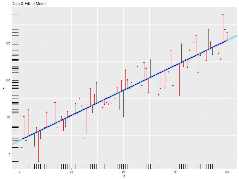
daDat <- data.frame(x=c(1, 2, 3, 4, 7, 8, 9, 10, 12, 13, 17, 18, 20, 21, 22, 23, 24, 27, 28, 29,
                        30, 31, 32, 34, 35, 36, 37, 40, 41, 42, 43, 46, 47, 48, 49, 50, 51, 52,
                        53, 54, 57, 59, 60, 61, 62, 63, 67, 68, 70, 71, 72, 73, 74, 77, 78, 79,
                        80, 81, 82, 84, 85, 86, 87, 90, 91, 92, 93, 96, 97, 98, 99, 100)
                    )                        # x-data
daDat$f <- 10+daDat$x*1.5                    # Function
daDat$e <- rnorm(daDat$x, mean=0, sd=15)     # Normally distributed errors           #### TRY THIS
#daDat$e <- runif(daDat$x, min=-40, max=40)  # Uniformly distributed errors          #### TRY THIS
#daDat$e <- runif(daDat$x, min=0, max=80)    # Uniformly distributed POSITIVE errors #### TRY THIS
daDat$y <- daDat$f + daDat$e                 # y-data
2.2. Compute the linear model
# x is the independent variable and y being the dependent one.
# data= simplifies the formula and makes future use of newdata= in 'predict' calls less painful.
daFit <- lm(y ~ x, data=daDat)
summary(daFit)
Call:
lm(formula = y ~ x, data = daDat)

Residuals:
    Min      1Q  Median      3Q     Max
-43.385 -11.517  -1.064  15.058  37.385

Coefficients:
            Estimate Std. Error t value Pr(>|t|)
(Intercept) 18.59925    4.72646   3.935 0.000194 ***
x            1.35089    0.08037  16.809  < 2e-16 ***
---
Signif. codes:  0 '***' 0.001 '**' 0.01 '*' 0.05 '.' 0.1 ' ' 1

Residual standard error: 19.82 on 70 degrees of freedom
Multiple R-squared:  0.8014,    Adjusted R-squared:  0.7986
F-statistic: 282.6 on 1 and 70 DF,  p-value: < 2.2e-16
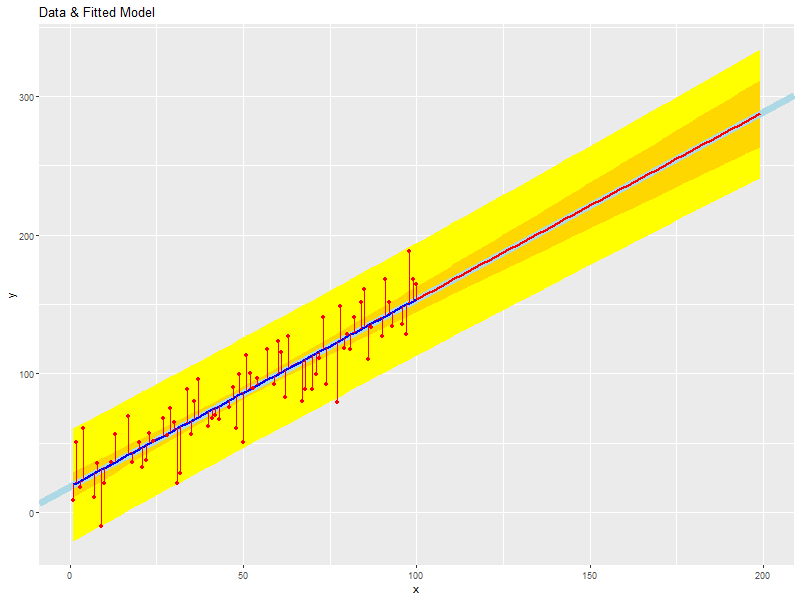
2.3. Plot Model
# plot the data with lines connecting points, draw the fitted line, mark the
# data points and fitted points with red dots and connect them with red lines.
ggplot(data=daDat, aes(x=x)) +
  geom_abline(intercept=coef(daFit)[1], slope=coef(daFit)[2], size=3, col='lightblue') +  # Fitted LINE
  geom_point(aes(y=y), col='red') +                                                       # Data points
  geom_line(aes(y=fitted(daFit)), col='blue', size=1) +                                   # Fitted SEGMENT
  geom_segment(aes(x=x, y=fitted(daFit), xend=x, yend=y), col='red') +                    # Error Bars
  labs(title='Data & Fitted Model', x='x', y='y')+                                        # Labels
  geom_rug(aes(y=y))                                                                      # Rugs for x and y data
2.4. Check our residuals for normally
2.4.1. With the Shpiro-Wilk test
# If p-value<0.1, then we reject the hypothesis that the residuals are normally distributed.
# NOTE: residuals(daFit) works on more "fit-like" objects than daFit$residuals
shapiro.test(residuals(daFit))
null device
          1

    Shapiro-Wilk normality test

data:  residuals(daFit)
W = 0.97823, p-value = 0.2458
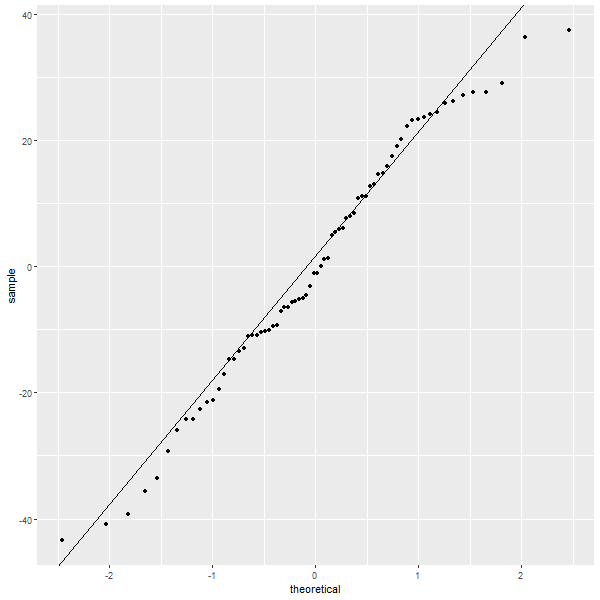
2.4.2. With a Q-Q plot
slope=(quantile(residuals(daFit),p=.75)-quantile(residuals(daFit),.25))/(qnorm(.75)-qnorm(.25))
intercept = quantile(residuals(daFit),.25) - slope*qnorm(.25)
ggplot() +
  geom_point(aes(sample=residuals(daFit)), stat="qq", distribution=qnorm) +   # Q-Q plot sf a normal
  geom_abline(intercept=intercept,slope=slope)                                # Q-Q plot *LINE* vs a normal
# Clean up temporary variables.
rm(slope, intercept)
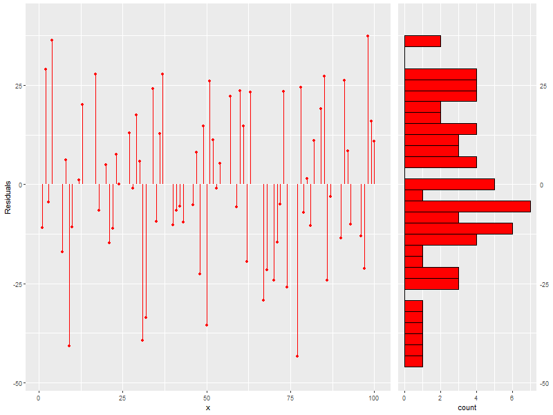
2.4.3. With a scatter plot (lines at mean, +sd, -sd, 2*sd, * -2*sd) and a histogram
daScat <- ggplot(data=daDat, aes(x=x)) +
  geom_point(aes(y=residuals(daFit)), col='red') +                               # Residuals
  geom_segment(aes(x=x, y=0, xend=x, yend=residuals(daFit)), col='red') +        # Residuals Bars
  labs(x='x', y='Residuals') +                                                   # Labels
  coord_cartesian(ylim = range(1.1*residuals(daFit)))

daHist <- ggplot() +
  geom_histogram(aes(x=residuals(daFit)), col='black', fill='red') +
  scale_x_continuous(position = "top") +
  theme(axis.ticks.y=element_blank(),
        axis.title.y=element_blank()
        ) +
  coord_flip(xlim = range(1.1*residuals(daFit)))


grid.arrange(daScat, daHist, ncol=2, nrow=1, widths=c(5, 2))
# Clean up temporary variables.
rm(daScat, daHist)
2.5. Prediction
2.5.1. Predict model values beyond our x-data
# Compute prediction intervals and confidence over the x-data and a an extended interval beyond the data...
newx <- data.frame(x=                                         # Compute new x points
                   seq(from=min(daDat$x),                     # Start at first data point:   x_min
                       to=max(daDat$x)+diff(range(daDat$x)),  # End one "range" beyond last: x_max+(x_max-x_min)
                       length.out=100))                       # Compute 100 points
tmpp <- predict(daFit, newdata=newx, interval="prediction")   # Compute prediction intervals
tmpc <- predict(daFit, newdata=newx, interval="confidence")   # Compute confidence intervals
newx <- data.frame(x=newx$x, fit=tmpc[,'fit'],                # Put everything in a data.frame
                   plwr=tmpp[,'lwr'], pupr=tmpp[,'upr'],
                   clwr=tmpc[,'lwr'], cupr=tmpc[,'upr'])
2.5.2. Plot our predictions
ggplot() +
  geom_ribbon(data=newx, aes(x=x, ymin=plwr, ymax=pupr), fill='yellow') +                 # prediction intervals
  geom_ribbon(data=newx, aes(x=x, ymin=clwr, ymax=cupr), fill='gold') +                   # confidence intervals
  geom_abline(intercept=coef(daFit)[1], slope=coef(daFit)[2], size=3, col='lightblue') +  # Fitted LINE
  geom_line(data=newx, aes(x=x, y=fit), col='red', size=1) +                              # Prediction SEGMENT
  geom_line(data=daDat, aes(x=x, y=fitted(daFit)), col='blue', size=1) +                  # Fitted SEGMENT
  geom_point(data=daDat, aes(x=x, y=y), col='red') +                                      # Data points
  geom_segment(data=daDat, aes(x=x, y=fitted(daFit), xend=x, yend=y), col='red') +        # Error Bars
  labs(title='Data & Fitted Model', x='x', y='y')
rm(newx, tmpp, tmpc)
2.6. Cleanup
rm(daDat, daFit)
3. Polynomial Regression
3.1. Example Data
# TRUE => fixed data, FALSE => randomly generated data.
if(TRUE) {
  daDat   <- data.frame(x=c(  0.000,  0.444,  0.888, 1.333, 1.777,  2.222,   2.666,  3.111,  3.555, 4.000),
                        f=c( -6.000, -2.208, -0.260, 0.370, 0.211, -0.211,  -0.370,  0.260,  2.208, 6.000),
                        e=c( -0.574, -0.193,  1.780, 1.260, 0.850,  1.233,  -1.589, -0.039, -1.774, 0.040),
                        y=c( -6.574, -2.401,  1.520, 1.631, 1.061,  1.021,  -1.960,  0.220,  0.433, 6.040))
} else {
  daDat   <- data.frame(x=seq(0, 4, length.out=20))  # x-data
  daDat$f <- with(daDat, x^3-6*x^2+11*x-6)           # Function
  daDat$e <- rnorm(daDat$x)                          # Error
  daDat$y <- daDat$f + daDat$e                       # y-data
}
3.2. Compute the polynomial models with progressively higher degree
maxFdeg <- 4                                            ######## TRY THIS: Value of 6 vs. 4
if(maxFdeg == 4) {
  ## For illustrative purposes we demonstrate hand coded formulas for the maxFdeg==4 case
  daFits <- list(lm(y ~ x,                    data=daDat),  # Degree 1 == simple linear regression
                 lm(y ~ x + I(x^2),           data=daDat),  # Note: The "I" function!
                 lm(y ~ x + I(x^2) + I(x^3),  data=daDat),
                 lm(y ~ poly(x, 4, raw=TRUE), data=daDat))  # Shorten the formulas with poly()
} else {
  ## This is how one generic fitting formulas can be constructed
  daFits <- lapply(1:maxFdeg, function (i) lm(y ~ poly(x, i, raw=TRUE), data=daDat))
}

daFits
null device
          1
`stat_bin()` using `bins = 30`. Pick better value with `binwidth`.
null device
          1
null device
          1
[[1]]

Call:
lm(formula = y ~ x, data = daDat)

Coefficients:
(Intercept)            x
     -3.065        1.582


[[2]]

Call:
lm(formula = y ~ x + I(x^2), data = daDat)

Coefficients:
(Intercept)            x       I(x^2)
    -3.8009       2.8245      -0.3106


[[3]]

Call:
lm(formula = y ~ x + I(x^2) + I(x^3), data = daDat)

Coefficients:
(Intercept)            x       I(x^2)       I(x^3)
     -6.971       15.872       -8.907        1.433


[[4]]

Call:
lm(formula = y ~ poly(x, 4, raw = TRUE), data = daDat)

Coefficients:
            (Intercept)  poly(x, 4, raw = TRUE)1  poly(x, 4, raw = TRUE)2  poly(x, 4, raw = TRUE)3  poly(x, 4, raw = TRUE)4
                -6.7171                  13.4953                  -5.9070                   0.2297                   0.1504
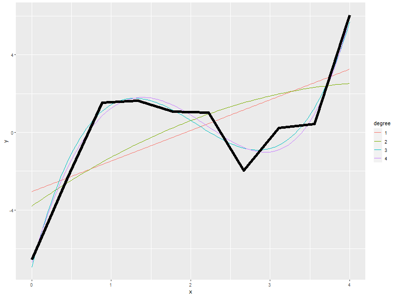
3.3. Plot Models
# Compute model values at 100 points between the min and max x values
newx  <- data.frame(x=seq(min(daDat$x), max(daDat$x), length.out=100))
newy  <- NULL
for(daFitDeg in 1:maxFdeg)
  newy  <- rbind(newy, data.frame(x=newx,
                                  degree=rep(daFitDeg, length(newx)),
                                  y=predict(daFits[[daFitDeg]], newdata=newx)))
newy$degree <- factor(newy$degree)
ggplot() +
  geom_line(data=newy,  aes(x=x, y=y,  col=degree)) +
  geom_line(data=daDat, aes(x=x, y=y), lwd=2)
3.4. Which fit is best?
# Use ANOVA to determine which fit seems best
do.call(anova, daFits)
null device
          1
Analysis of Variance Table

Model 1: y ~ x
Model 2: y ~ x + I(x^2)
Model 3: y ~ x + I(x^2) + I(x^3)
Model 4: y ~ poly(x, 4, raw = TRUE)
  Res.Df    RSS Df Sum of Sq       F    Pr(>F)
1      8 55.775
2      7 53.788  1     1.987  2.2840 0.1911087
3      6  4.917  1    48.871 56.1845 0.0006681 ***
4      5  4.349  1     0.567  0.6523 0.4559873
---
Signif. codes:  0 '***' 0.001 '**' 0.01 '*' 0.05 '.' 0.1 ' ' 1
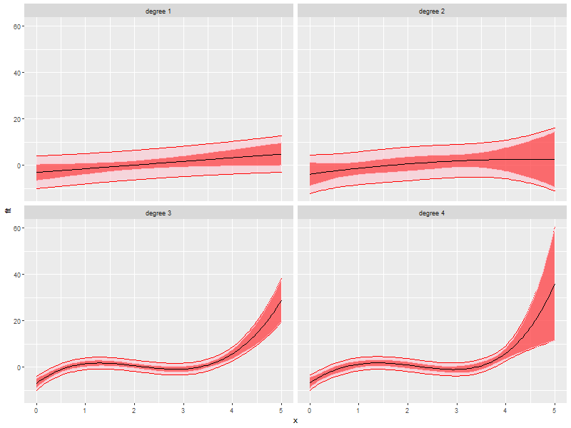
3.5. Prediction intervals and confidence intervals
newx  <- data.frame(x=seq(from=min(daDat$x),
                          to=max(daDat$x)+diff(range(daDat$x))/4,
                          length.out=100))
newy  <- NULL
for(daFitDeg in 1:maxFdeg) {
  tmpp <- predict(daFits[[daFitDeg]], newdata=newx, interval="prediction")
  tmpc <- predict(daFits[[daFitDeg]], newdata=newx, interval="confidence")
  newy  <- rbind(newy, data.frame(x      = newx,
                                  degree = rep(daFitDeg, length(newx)),
                                  fit    = tmpp[,'fit'],
                                  pLow   = tmpp[,'lwr'],
                                  pUp    = tmpp[,'upr'],
                                  cLow   = tmpc[,'lwr'],
                                  cUp    = tmpc[,'upr']))
}
newy$degree <- factor(paste('degree', newy$degree))
ggplot(newy, aes(x=x, y=fit, group=degree)) +
  facet_wrap(~degree, ncol=2) +
  geom_ribbon(aes(ymin=pLow, ymax=pUp), alpha=.5, fill='pink', col='red') +
  geom_ribbon(aes(ymin=cLow, ymax=cUp), alpha=.5, fill='red', col='pink') +
  geom_line()
4. Non-Linear Regression
4.1. Example Data
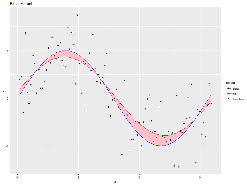
## Make up some data: y=sin(x)+e where e is random (normal or uniform)
numPts   <- 100
daDat    <- data.frame(x=1:numPts/(numPts/20*pi))    # x-data
daDat$f  <- sin(daDat$x)                  # Function
daDat$e  <- rnorm(daDat$x, mean=0, sd=.5) # Identically distributed Normal Error
#daDat$e <- runif(daDat$x, -1, 1)         # Identically distributed Uniform Error
#daDat$e <- runif(daDat$x, 0, 1)          # Identically distributed, but asymmetric, Uniform Error
#daDat$e <- daDat$x*rnorm(daDat$x, sd=.5) # Non-Identically distributed Normal Error
daDat$y  <- daDat$f + daDat$e             # y-data
4.2. Compute non-linear model
# Compute the non-linear model
# Independent variable of x, dependent variable of y, and function of a*sin(b*x+c)+d
daFit   <- nls(y~a*sin(b*x+c)+d,           # Model formula
               data=daDat,                 # data= simplifies the formula argument & future predict calls
               start=list(a=1,b=1,c=0,d=0) # Initial conditions (we set them to the true model values)
               )

summary(daFit)
null device
          1

Formula: y ~ a * sin(b * x + c) + d

Parameters:
  Estimate Std. Error t value Pr(>|t|)
a  0.82561    0.06216  13.282   <2e-16 ***
b  0.94955    0.04079  23.277   <2e-16 ***
c  0.11286    0.15223   0.741    0.460
d  0.04486    0.04312   1.040    0.301
---
Signif. codes:  0 '***' 0.001 '**' 0.01 '*' 0.05 '.' 0.1 ' ' 1

Residual standard error: 0.4305 on 96 degrees of freedom

Number of iterations to convergence: 4
Achieved convergence tolerance: 2.464e-06
4.3. Plot Model
# This plot is not terribly useful for the practicing data modeler as one wouldn't be
# modeling the data in the first place if the true model from which the data was
# generated available!  That said, it is an interesting way to explore how pushing
# the envelope of the various theoretical requirements impacts the accuracy of the
# fit (Try adding one sided, positive errors or non-normal ones).

daDat$fit <- fitted(daFit)                          # Fitted valeus -> a data.frame

ggplot(daDat) +
  geom_ribbon(aes(x=x,
                  ymin=pmin(daDat$f, daDat$fit),
                  ymax=pmax(daDat$f, daDat$fit)),
              fill='pink') +
  geom_line(aes(x=x, y=f,   col='function')) +      # Note: col is an aes!
  geom_point(aes(x=x, y=y,  col='data')) +
  geom_line(aes(x=x, y=fit, col='fit')) +
  labs(title='Fit vs Actual',
       x='x',
       y='y') +
  scale_color_manual(values=c("black",     "red", "blue"))