HP-15C Tips & Tricks
| Author: | Mitch Richling |
| Updated: | 2025-05-16 |
| Generated: | 2025-05-16 |
Copyright © 2025 Mitch Richling. All rights reserved.
Table of Contents
1. Introduction
This document contains computational recipes for the HP-15C. Most of these items fall into one of the following categories:
- Some tricky behavior of the 15C
- An efficient way to preform some computation on the 15C
- Illustrate a neat way to solve a problem – not necessarily 15C specific
2. Triangles
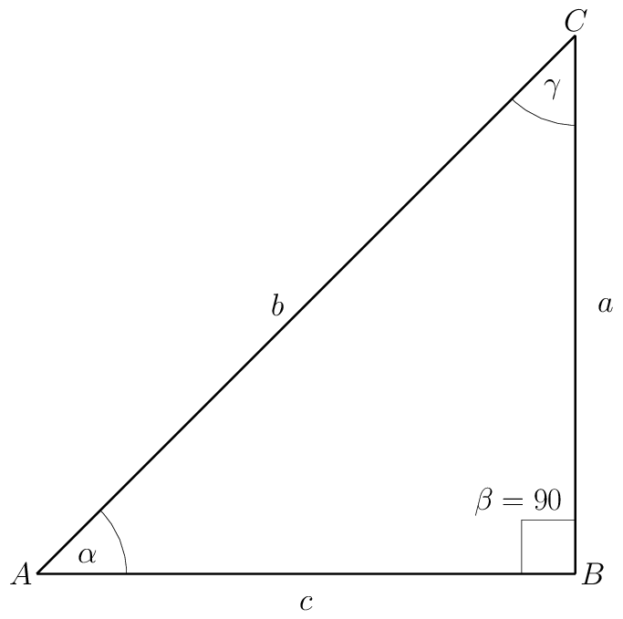
2.1. Right Triangle: Known Hypotenuse & angle
This item illustrates the different behavior of →R and →P when complex mode (flag 9 set) is enabled.

With \(b=5\) and \(\alpha=30\).
2.1.1. Complex Mode
If the calculator is in complex mode (Flag F 8 set):
| g DEG | Put calculator in degree mode (if necessary) |
| 5 ENTER 3 0 f I f →R | Enter complex number \(5\angle30\) (length of \(b\) and \(\alpha\) angle) |
\(c\) is on the real stack at X, and \(a\) is on the complex stack at X.
2.1.2. Real Mode
If the calculator is not in complex mode (Flag F 8 clear):
| g DEG | Put calculator in degree mode (if necessary) |
| 3 0 ENTER 5 f →R | Enter \(\alpha\) and \(b\) on the stack, and convert to rectangular |
\(c\) is on the stack at X, and \(a\) is on the stack at Y.
2.2. Right Triangle: Known Legs (the 2D HYPOT function)
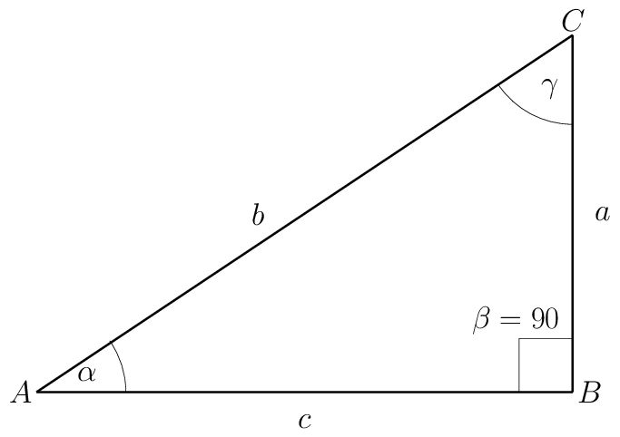
Like the previous item, this one also illustrates the different behavior of →R and →P when complex mode (flag F 8 set) is enabled. In addition, this item illustrates the most efficient way to compute the 2D \(\mathrm{HYPOT}\) function.
The 2D \(\mathrm{HYPOT}\) function is defined as \(\mathrm{HYPOT}(x,y)=\sqrt{x^2+y^2}\). The function is so named because its value is the length of the hypotenuse of a triangle with leg lengths of \(x\) & \(y\). A slight modification to the triangle solution technique below gives us a method to compute \(\mathrm{HYPOT}\) with the fewest keystrokes. In particular, when computing \(\mathrm{HYPOT}(x,y)\) we don't need to insure the calculator is in degree mode – i.e. to compute \(\mathrm{HYPOT}(x,y)\) we can skip the first step in each of the procedures below. For how to compute the generalized \(\mathrm{HYPOT}\) function, see HYPOT below.

With \(c=4\) and \(b=3\).
2.2.1. Complex Mode
If the calculator is in complex mode (Flag F 8 set):
| g DEG | Put calculator in degree mode (if necessary) |
| 4 ENTER 3 f I | Enter complex number \(4+3i\) |
| g →P | Convert to polar form. |
\(b\) is the real stack at X, and \(\alpha\) is on the complex stack at X.
2.2.2. Real Mode
If the calculator is not in complex mode (Flag F 8 clear):
| g DEG | Put calculator in degree mode (if necessary) |
| 3 ENTER 4 g →P | Enter \(b\) & \(c\) on the stack, and convert to polar |
\(b\) is the stack at X, and \(\alpha\) is on the stack at Y.
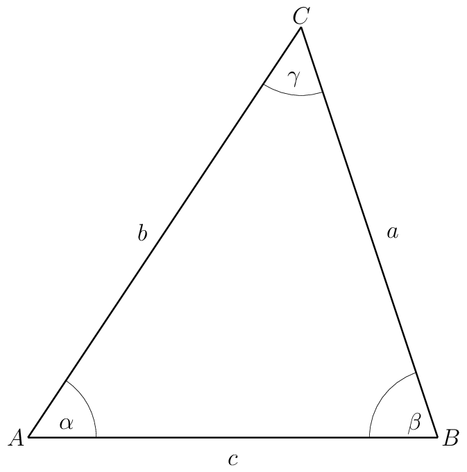
2.3. General Triangle: SAS (Side Angle Side)
The way the HP-15C works with complex numbers exposes the real & imaginary parts to the user for individual manipulation. For example the HP-15C has no Re,
Im, or conj functions because they are simply unnecessary. This design choice makes it simple to change the sign of the real part of a complex number on
the HP-15C with a single keystroke! Most calculators require several keystrokes to achieve the same task. For example, on the HP-42S we might use a sequence
like [COMPLEX] [X<>Y] [CHS] [X<>Y] [COMPLEX] to change the sign of the real part of a complex number.
In the sequence below we change the sign of the real part of a complex number with a single keystroke (step 4 below). We do this to transform the complex number's argument to the supplementary angle.

With \(b=5\), \(\alpha=30\), and \(c=4\).
| g DEG | Put calculator in degree mode (if necessary) |
| 5 ENTER 3 0 f I f →R | Enter complex number \(5\angle30\) (length of \(b\) and \(\alpha\) angle) |
| 4 - | Subtract \(4+0i\) (the length of \(c\)). Gives side \(a\) as a complex number |
| CHS | Changing the real part sign transforms the complex angle to the supplementary angle. |
| →P | Convert to polar form. |
\(a\) will be on the real stack at X, and \(\beta\) will be on the complex stack at X.
3. Lines
3.1. Equation of line given two points
The mathematical idea behind how this works is that linear regression with only two points produces the equation of the interpolating line.
This works on any calculator that can do linear regression, but the process is particularly efficient on the 15C. For example, the entire process on the
HP-15C requires only 7 keystrokes beyond data entry; however, on the fx-5800P (my favorite algebraic scientific calculator) it takes 18 keystrokes ([mode]
[4] [function] [5] [1] [2] [EXE] x1 [EXE] x2 [EXE] [UP] [UP] [RIGHT] y1 [EXE] y2 [EXE] [FUNCTION] [6] [2] [1]).
Find the equation of the line passing through \((2,3)\) and \((5,2)\) in slope-intercept form (i.e. \(y=mx+b\)).
| f CLR_Σ | Clear statistical registers (if necessary) |
| 3 ENTER 2 Σ+ | Enter first point (note y goes in first) |
| 2 ENTER 5 Σ+ | Enter second point |
| f L.R. | Compute the line |
The value for \(m\) is in Y, and value for \(b\) is in X.
3.2. Linear Interpolation & extrapolation (applied to Fahrenheit/Celsius Conversion)
This item is a continuation of the previous one, but this time we are interested in computed values on the line instead of the equation – i.e. we are interested in linear interpolation! Like in the previous topic, this concept works with any calculator capable of linear regression; however, the process is so cumbersome on many modern calculators that it's simply not worth the effort. On the Casio fx-5800P it takes 18 keystrokes (see: previous topic) to set up the interpolation, and 7 keystrokes ([FUNCTION] [7] [2] [DOWN] [DOWN] [DOWN] [ŷ]) to compute an interpolated value. Compare this to 7 keystrokes to set up the line, and 2 keystrokes to compute a value on the HP-15C. This is where the HP-15C shines.
Suppose we have several Fahrenheit values we need to convert to Celsius. We know the two values have a linear relationship, and we also remember the corresponding values in each system for the freezing and boiling points of water. In particular 0 Celsius corresponds to 32 degrees Fahrenheit, and 100 Celsius corresponds to 212 Fahrenheit. We wish to convert 68, 70, & 72 degrees Fahrenheit to Celsius.
| f CLR_Σ | Clear statistical registers (if necessary) |
| 0 ENTER 3 2 Σ+ | Enter first known point |
| 1 0 0 ENTER 2 1 2 Σ+ | Enter second known point |
| 6 8 f ŷ,r | The celsius value is on the stack at X |
| 7 0 f ŷ,r | The celsius value is on the stack at X |
| 7 2 f ŷ,r | The celsius value is on the stack at X |
For non-linear interpolation see: non-linear interpolation.
4. 2D vectors
4.1. Vector Sums
The obvious approach to summing a series of 2D vectors is to use complex number arithmetic. That approach works just fine, but we can use the HP-15C's statistical capabilities to do the same computation with fewer keystrokes when working with more than 2 vectors.
Sum the following four vectors: \((2,3), (5,2), (7,7), (3,5)\). In what follows we use the statistical registers in reverse because entry is less error prone.
| f CLR_Σ | Clear statistical registers (if necessary) |
| 2 ENTER 3 Σ+ | Enter first vector |
| 5 ENTER 2 Σ+ | Enter second vector |
| 7 ENTER 7 Σ+ | Enter third vector |
| 3 ENTER 5 Σ+ | Enter fourth vector |
| RCL 3 | Sum of the \(y\) components |
| RCL 5 | Sum of the \(x\) components |
The sum of the \(x\) components will be in X, and \(y\) sum will be in Y .
4.2. Angle between vectors
4.2.1. Two Dimensional Case
This item is more about pointing out that we can find the angle between two vectors in 2D using complex arithmetic instead of the traditional vector angle formula. This works on any calculator supporting both polar & rectangular complex arithmetic.
Find the angle between the vectors \((2,3)\) and \((3,2)\).
| g DEG | Put calculator in degree mode (if necessary) |
| 2 ENTER 3 f I | Enter complex number \(2+3i\) for the first vector |
| 3 ENTER 2 f I | Enter complex number \(3+2i\) for the first vector |
| ÷ →P | Divide and convert to polar form |
The angle is on the complex stack at X.
4.2.2. Higher Dimensional Case
When working with 3, or more, component vectors we can use the statstical registers.
| f CLR_Σ ( \(x_i\) ENTER \(y_i\) f Σ+ …) RCL 7 RCL 4 RCL 6 × √x ÷ |
For example find the angle between the following two vectors: \((2,3,5)\) & \((6,7,8)\).
| g DEG | Put calculator in degree mode (if necessary) |
| f CLR_Σ | Clear statistical registers (if necessary) |
| 2 ENTER 6 Σ+ | Enter first coordinates for each vector |
| 3 ENTER 7 Σ+ | Enter second coordinates for each vector |
| 5 ENTER 8 Σ+ | Enter last coordinates for each vector |
| RCL 7 RCL 4 RCL 6 × √x ÷ | Compute the angle |
The angle will be in X.
5. General HYPOT Function
The \(\mathrm{HYPOT}(x,y)\) function may be generalized to \(n\mathrm{-vectors}\) like so:
\[\mathrm{HYPOT}(\vec{x})=\sqrt{\sum_{i=1}^n x_i}\]
Note this is nothing more than the Euclidean Norm (2-norm) usually written \(\left\Vert\vec{x}\right\Vert_2\) or simply \(\left\Vert\vec{x}\right\Vert\).
The most efficient way to compute this function when \(n=2\) is provided in a previous topic.
When \(n=3\) the best sequence is
| \(x_1\) ENTER × \(x_2\) ENTER × + \(x_3\) ENTER × + √x |
When \(n>3\) the best sequence is
| f CLR_Σ ( \(x_i\) Σ+ …) RCL 4 √x |
6. Non-Linear Regression & Interpolation
Most modern calculators can do several types of regression. Many older calcualtors supported four: linear, logarithmic, exponential, and power. One of the reason these four were supported early on is that they can be computed from summary statstics via logarithmic/exponential data transformations. This allowed them to be implimented on calcualtors with very little memory.
6.1. Classic Non-Linear Regression
Almost all scientific calculators support the folling four types of regression:
| Regression Type | Formula |
|---|---|
| linear | y=ax+b$ |
| exponential | y=be^{ax}$ |
| logarithmic | y=aln(x)+b$ |
| power | y=bx^{ax}$ |
Unfortunately the HP-15C only supports linear regression out of the box. So we must do a bit more work to compute the others. Luckily, it's not hard – we just need to transform the data as we enter it, and transform answers we extract.
| Regression Type | Data Entry Procedure | Regression Coefficients | Predictiction |
|---|---|---|---|
\(b\) X and \(a\) Y. |
\(y\) given \(x\) | ||
| linear | \(y_i\) ENTER \(x_i\) Σ+ | f L.R. | \(x\) ŷ,r |
| logarithmic | \(y_i\) ENTER \(x_i\) g LN Σ+ | f L.R. | \(x\) g LN ŷ,r |
| exponential | \(y_i\) g LN \(x_i\) Σ+ | f L.R. eˣ | \(x\) ŷ,r eˣ |
| power | \(y_i\) g LN \(x_i\) g LN Σ+ | f L.R. eˣ | \(x\) g LN ŷ,r eˣ |
6.2. Logarithmic Interpolation (Non-Linear Interpolation)
We can use the same method employed with linear interpolation with the non-linear regression methods mentioned previously. For me the most common non-linear regression I preform is logarithmic.
Suppose we have two points, \((x_1, y_1)\) and \((x_2, y_2)\), that we know are on a curve of the form \(y=m\cdot\ln(x)+b\). As a practical example, it might be the case that we have two voltage/current points on a diode V-I curve and we wish to know the coefficients in the Shockley diode equation.
For this example, let us suppose \((x_1, y_1)=(2,3)\) and \((x_2, y_2)=(5,2)\)
| f CLR_Σ | Clear statistical registers (if necessary) |
| 3 ENTER 2 g LN Σ+ | Enter first point (note y goes in first) |
| 2 ENTER 5 g LN Σ+ | Enter second point |
| L.R. | Compute the coefficients |
The value for \(m\) is in Y, and value for \(b\) is in X.
This technique is quite general and we need not limit ourselves to logarithmic transformations. For example, we can replace \(\ln(x)\) with any function, \(g(x)\), so long as \(g(x)\) is monotone on the interval \([x_1, x_2]\). For example, we could fit \(y=m\cdot\sin(x)+b\) to the points \((0,1)\) & \((1.5, 2)\) – because \(\sin(x)\) is monotone on \([0, 1.4]\).
7. 2D Normal Equations
Let \( A\in\mathbb{R}^{m\times 2} \) be a two column real matrix with \( m>2 \). We wish to compute \( N = A^T A \). We can use the statistical functions to compute the matrix and/or it's determinant. This technique requires fewer keystrokes, and also consumes no matrix storage. That said, it uses the statistical registers (R 2-R 7).
For this example, let us suppose \[ A = \left[ {\begin{array}{cc} 1 & 2 \\ 3 & 4 \\ 5 & 6 \\ \end{array} } \right] \]
| f CLR_Σ | Clear statistical registers (if necessary) |
| 1 ENTER 2 Σ+ | Enter first row |
| 3 ENTER 4 Σ+ | Enter second row |
| 5 ENTER 6 Σ+ | Enter third row |
| RCL 6 | \( N_{1,1} \). |
| RCL 7 | \( N_{1,2} \) & \( N_{2,1} \) |
| RCL 4 | \( N_{2,2} \). |
Note we can compute \( \det(N) \) like this: RCL 6 RCL 4 × RCL 7 g x² -
8. HP 15c CE Stuff
I have one 15c from the mid 80's, and three 15 CE (collector's edition) units from 2023.
8.1. Diagnostics & Easter Eggs
- Turn the Calculator off.
- Hold g and ENTER, press ON. Release ON, and then ENTER & g.
- On screen see
1.L 2.C 3.H - We can now do a few things:
- Press 1 to test the LCD
- Press 2 for a firmware checksum
- Press 3 to test the keyboard
- Press 4 for Easter Eggs!
- On screen see
15 15.2 16 - At this point we can do three things:
- Press eˣ for the factory settings. Ordinary HP-15c CE mode with 96 registers.
- Press yˣ for the 2X memory mode with 192 registers.
- Press 7 for the HP-16C mode.
- On screen see
8.2. Voyager Save
- Turn the Calculator off.
- Hold f and ENTER, press ON. Release ON, and then ENTER & f.
- This will put the calculator in USB HID mode.
I have been keeping my CE in 2X memory mode because I find myself needing a bit more RAM for program and matrix storage.
9. Meta Data
The primary URL for this page: https://richmit.github.io/voyager/hp15-tips.html
The org mode file for this page: https://github.com/richmit/voyager/blob/main/docs/hp15-tips.org
The HTML file for this page: https://github.com/richmit/voyager/blob/main/docs/hp15-tips.html
The github repository housing this content: https://github.com/richmit/voyager/