MRKISS Library
MR RK (Runge-Kutta) KISS (Keep It Super Simple)
| Author: | Mitch Richling |
| Updated: | 2025-09-21 13:15:49 |
| Generated: | 2025-09-21 13:15:50 |
Copyright © 2025 Mitch Richling. All rights reserved.
Table of Contents
- 1. Introduction
- 2. Vocabulary & Definitions
- 3. Features & Requirements
- 4. Defining Runge-Kutta Methods in
MRKISS - 5. Predefined Runge-Kutta Methods in
MRKISS - 6. Providing ODE Equations For Solvers
- 7. High Level Solvers
- 8. Low Level, One Step Solvers
- 9. Utilities
- 10. Quick Start – The Absolute Minimum
- 11. Using
MRKISSIn Your Projects - 12.
MRKISSTesting - 13. FAQ
- 13.1. What's with the name?
- 13.2. Why Fortran
- 13.3. Why did you write another ODE solver when so many good options exist?
- 13.4. Why don't you use package XYZ?
- 13.5. What are those zotero links in the references?
- 13.6. Are high order RK methods overkill for strange attractors?
- 13.7. I need a more comprehensive solution. Do you have advice?
- 13.8. I need something faster. Do you have advice?
- 13.9. It seems like things are used other than Fortran. Are there really no external dependencies?
- 13.10. What is a "Release"? How is it different from what's on
HEAD? - 13.11. What platforms are known to work?
1. Introduction
MRKISS is a simple, tiny library with zero dependencies[*] that aims to make it easy to use
and experiment with explicit Runge-Kutta methods.
From a feature standpoint this library doesn't do anything you can't find in more comprehensive packages like
SUNDIALS or Julia's
DifferentialEquations.jl; however, it has the rather charming feature of being super simple and self contained. This makes it ideal for sharing results and
code with others without asking them to recreate my technical computing environment or learn about new software. It also makes it easy to get things up and
and running quickly when moving to a new supercomputer, cloud, or HPC cluster.
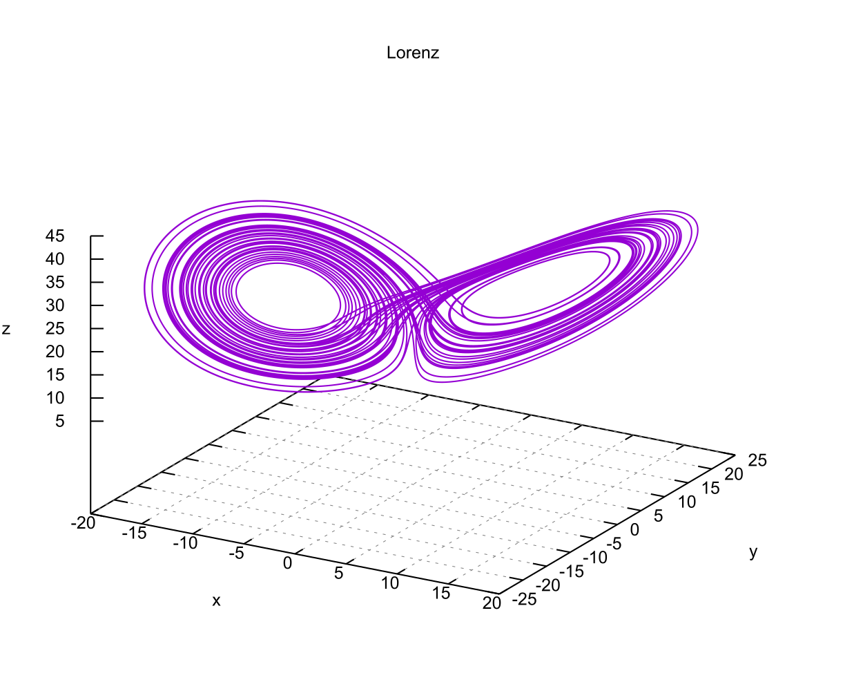
Here is a complete example in 23 lines that solves Lorenz's system and generates a CSV file of the results.
program minimal

  use :: mrkiss_config,      only: rk, istats_size
  use :: mrkiss_solvers_nt,  only: fixed_t_steps
  use :: mrkiss_utils,       only: print_solution
  use :: mrkiss_erk_kutta_4, only: a, b, c

  implicit none (type, external)

  real(kind=rk), parameter :: y_iv(3)  = [1.0_rk, 0.0_rk, 0.0_rk]
  real(kind=rk), parameter :: param(3) = [10.0_rk, 28.0_rk, 8.0_rk/3.0_rk]
  real(kind=rk), parameter :: t_end    = 50.0_rk

  real(kind=rk)            :: solution(7, 10000)
  integer                  :: status, istats(istats_size)

  call fixed_t_steps(status, istats, solution, eq, y_iv, param, a, b, c, t_end_o=t_end)
  call print_solution(status, solution, filename_o="minimal.csv")

contains

  subroutine eq(status, dydt, y, param)
    integer,          intent(out) :: status
    real(kind=rk),    intent(out) :: dydt(:)
    real(kind=rk),    intent(in)  :: y(:), param(:)
    dydt = [ param(1)*(y(2)-y(1)), y(1)*(param(2)-y(3))-y(2), y(1)*y(2)-param(3)*y(3) ]
    status = 0
  end subroutine eq

end program minimal
You can check out a couple larger examples:
If you just want to jump in, then take a look at the Quick Start section.
2. Vocabulary & Definitions
Before discussing the software, it is best if we define the problem we are solving and fix some definitions and notation – notation that is used throughout the source code and documentation.
Please note that the material below deviates from the standard presentation of Runge-Kutta methods and the Butcher tableau. In particular we dispense with separate \(\mathbf{b}\) vectors per method, the silly hats, and express most of the computations in terms of linear algebra.
Solving an ODE (Ordinary Differential Equation):
We wish to compute values for an unknown function \(\mathbf{y}:\mathbb{R}\rightarrow\mathbb{R}^n\) on some interval \([t_\mathrm{iv}, t_\mathrm{max}]\) given an initial value \(\mathbf{y}(t_\mathrm{iv})=\mathbf{y_\mathrm{iv}}\) and an implicit equation involving \(t\), \(\mathbf{y}\), and it's derivatives:
\[ \mathbf{y}' = \mathbf{f}(t, \mathbf{y}) \]
The expression above may be written in component form as:
\[ \frac{\mathrm{d}\mathbf{y}}{\mathrm{d}t} = \mathbf{f}(t, \mathbf{y}) = \left[\begin{array}{c} \frac{\mathrm{d}y_1}{\mathrm{d}t} \\ \vdots \\ \frac{\mathrm{d}y_n}{\mathrm{d}t} \\ \end{array}\right] = \left[\begin{array}{c} f_1(t, \mathbf{y}) \\ \vdots \\ f_n(t, \mathbf{y}) \\ \end{array}\right] = \left[\begin{array}{c} f_1(t, [y_1, \cdots, y_n]^\mathrm{T}) \\ \vdots \\ f_n(t, [y_1, \cdots, y_n]^\mathrm{T}) \\ \end{array}\right] \]
If the function \(\mathbf{f}(t, \mathbf{y}) \) doesn't actually depend on \(t\), then the ODE is said to be Autonomous.
We define an \(s\)-stage embedded explicit Runge-Kutta method via a set of coefficients organized into a Butcher tableau:
\[ \begin{array}{l|llll} c_1 & a_{1,1} & a_{1,2} & \dots & a_{1,s} \\ c_2 & a_{2,1} & a_{2,2} & \dots & a_{2,s} \\ c_3 & a_{3,1} & a_{3,2} & \dots & a_{3,s} \\ \vdots & \vdots & \vdots & \ddots & \vdots \\ c_s & a_{s,1} & a_{s,2} & \dots & a_{s,s} \\ \hline \rule{0pt}{12pt} & b_{1,1} & b_{1,2} & \dots & b_{1,s} \\ & \vdots & \vdots & \ddots & \vdots \\ & b_{m,1} & b_{m,2} & \dots & b_{m,s} \\ \end{array} \]
We reference the blocks of the tableau as (Note \(\mathbf{b}\) is transposed compared to the tableau):
\[ \mathbf{a} = \begin{bmatrix} a_{1,1} & a_{1,2} & \dots & a_{1,s} \\ a_{2,1} & a_{2,2} & \dots & a_{2,s} \\ a_{3,1} & a_{3,2} & \dots & a_{3,s} \\ \vdots & \vdots & \ddots & \vdots \\ a_{s,1} & a_{s,2} & \dots & a_{s,s} \end{bmatrix} \,\,\,\,\,\,\,\, \mathbf{c} = \begin{bmatrix} c_{1} \\ c_{2} \\ c_{3} \\ \vdots \\ c_{s} \end{bmatrix} \,\,\,\,\,\,\,\, \mathbf{b} = \begin{bmatrix} b_{1,1} & \dots & b_{1,m} \\ b_{2,1} & \dots & b_{2,m} \\ b_{3,1} & \dots & b_{3,m} \\ \vdots & \ddots & \vdots \\ b_{s,1} & \dots & b_{s,m} \end{bmatrix} = \begin{bmatrix} \vert & & \vert \\ \mathbf{b}_1 & \dots & \mathbf{b}_m \\ \vert & & \vert \\ \end{bmatrix} \]
Note we use \(\mathbf{b}_i\) with an index to indicate the \(i\)-th column of the matrix, and \(b_{i,j}\) to indicate the \(i,j\)-th element of the matrix.
The word embedded is used to indicate that the tableau actually defines \(m\) Runge-Kutta methods – one for each column of \(\mathbf{b}\). The most common cases are \(m=1\) and \(m=2\) with the first being most commonly used for simple, fixed step size solvers and second most commonly used for adaptive step size solvers.
We say the overall number of stages for the entire embedded method is \(s\), but the number of stages required for an individual method associated with a column of \(\mathbf{b}\) might be lower if that column has trailing zeros. If a column has \(k\) trailing zeros the Runge-Kutta method associated with that column has\(s-k\) stages.
Our goal is to compute values of \(\mathbf{y}(t)\) for \(t\in[t_\mathrm{iv}, t_\mathrm{max}]\). We are given the value of \(\mathbf{y}(t_\mathrm{iv})\). So we define a small, positive value \(\Delta{t}\in\mathbb{R}\), and attempt to find \(\mathbf{\Delta{y}}\) such that \(\mathbf{y}(t_\mathrm{iv})+\mathbf{\Delta{y}}\approx\mathbf{y}(t_\mathrm{iv}+\Delta{t})\).
We begin by defining an \(s\times s\) matrix \(\mathbf{k}\):
\[ \mathbf{a} = \begin{bmatrix} k_{1,1} & k_{1,2} & \dots & k_{1,s} \\ k_{2,1} & k_{2,2} & \dots & k_{2,s} \\ k_{3,1} & k_{3,2} & \dots & k_{3,s} \\ \vdots & \vdots & \ddots & \vdots \\ k_{s,1} & k_{s,2} & \dots & k_{s,s} \end{bmatrix} = \begin{bmatrix} \vert & & \vert \\ \mathbf{k}_1 & \dots & \mathbf{k}_s \\ \vert & & \vert \\ \end{bmatrix} \]
Using
\[ \mathbf{k}_i = \mathbf{f}\left(t + c_i \Delta{t},\, \mathbf{y} + \Delta{t} \mathbf{k}_{1..s,1..i} \mathbf{a}_{1..i,1..i} \right) \]
Explicit methods, which are the focus of MRKISS, have \(c_1=0\) and \(a_{ij}=0\) for \(i\le j\). Therefore
\(\mathbf{k}_1 = \mathbf{f}(t,\, \mathbf{y})\), and each subsequent \(\mathbf{k}\) value may be computed in sequence.
Each column of \(\mathbf{k}\mathbf{b}\) forms a \(\mathbf{\Delta{y}}\) we can use to approximate \(\mathbf{y}(t_\mathrm{iv}+\Delta{t})\):
\[ \mathbf{k}\mathbf{b} = \begin{bmatrix} \vert & & \vert \\ \mathbf{\Delta{y}}_1 & \dots & \mathbf{\Delta{y}}_m \\ \vert & & \vert \\ \end{bmatrix} \]
If we use \(\mathbf{\Delta{y}}_1\) to approximate \(\mathbf{y}(t_\mathrm{iv}+\Delta{t})\), then we can use \(\mathbf{\Delta{y}}_2\) to approximate the error like this:
\[\vert\mathbf{\Delta{y}}_1 - \mathbf{\Delta{y}}_2 \vert\]
We say that a Runge-Kutta method is of order \(p\in\mathbb{Z_+}=\{i\in\mathbb{Z}\,\,\vert\,\,i>0\}\) if the error at each step is on the order of \(\mathcal{O}(\Delta{t}^{p+1})\) and the accumulated error of multiple steps is of order \(\mathcal{O}(\Delta{t}^{p})\). This abuse of big-O terminology is traditionally also extended to an abuse of big-O notation by saying the Runge-Kutta method is \(\mathcal{O}(p)\).
3. Features & Requirements
The IVPs I work with are generally pretty well behaved
- Non-stiff
- Time forward (\(\Delta{t} \ge 0\))
- Defined by a small (<50) set of equations expressible in closed form.
Typical examples are strange attractors and systems related to chaotic science models from celestial/classical mechanics, population dynamics, oscillating chemical reactions, and electronic circuits. My motivation for solving IVPs generally revolve around generative art and visualization. You will actually see this in the code and feature set of the library.
Things I care about
- Simple to use for simple problems.
- Graceful response to evaluation failure in derivative functions
- A good selection of predefined RK methods
- Standard, adaptive step solver with programmable step processing:
- Easy deployment & sharing
- Easy to compile and tune for a new hardware architectures.
- Zero external dependencies[*] except a Fortran compiler.
- 100% standard Fortran that works with various compilers.
- Simple text output that can be compressed and sent back home or shared with others.
- Runge-Kutta Research
- Try out new RK methods by simply feeding the solvers a Butcher tableau.
- Directly accessible one step routines for assembling custom solvers.
- Simple code flow to facilitate instrumentation and deep runtime analysis and reporting.
- Individual access to each method in an embedded tableau, and control over how each is used.
- Machine readable butcher tableau data and Maple worksheets to process that data.
- A few of the RK methods included are of historical or research interest – not necessarily very practical.
- Generative art and visualization functionality
- Solutions include derivative values for visualization tools.
- Programmable step processing tuned for visualization problems.
- Stopping integration. Examples:
- If the solution curve is too long in \(\mathbf{y}\)-space
- If the step delta, or some components of it, are too long in \(\mathbf{y}\)-space
- If the solution has returned to the IV
- If the solution intersects itself
- Provide an alternate \(\Delta{t}\) and redo the step based on some condition.
- Trigger a bisection search for a \(\Delta{t}\) fitting some condition based on t-space and/or \(\mathbf{y}\)-space. Examples:
- Find \(\Delta{t}\) so that \(\Delta{\mathbf{y}}\), or some components of it, are the perfect length.
- Find where a step crosses over a boundary in space (ex: root finding)
- Find where a step approaches closest to a point (ex: like the problem's IV)
- Stopping integration. Examples:
- Easy to use, hardwired methods for fixed step size visualization use cases:
- Fixed \(t\) step size solvers
- Fixed \(\mathbf{y}\) step size solver with hard bounds on length error
- Fixed \(\mathbf{y}\) step size solver with soft bounds on length error
- Interpolate entire solutions to new time points (Hermite & linear).
Things that may weird you out
Derivative function computation dominates the compute time for many applications. This observation has had tremendous influence on the development of IVP
numerical techniques and related software. For the IVPs we are interested in the derivative functions are quite simple and the Runge-Kutta computations
themselves generally dominate the computation time. This changes things quite dramatically. For example, techniques like embedded polynomial schemes for
intrastep interpolation designed to minimize function evaluation may actually perform worse than simply making more Runge-Kutta steps for our problems! As
another example, performing iterative algorithms, like bisection, directly on the Runge-Kutta method itself is quite practical. Keeping this in mind will
reduce the number of "WTH?!?!" moments you have while reading the code, and will keep you from applying some features, like fixed_y_steps(), to
problems that do have difficult derivatives to compute.
While MRKISS provides comprehensive support for detecting and forwarding runtime errors, it doesn't do much
programmer error checking. For example, the code doesn't double check that the programmer has provided appropriate arguments for routines.
4. Defining Runge-Kutta Methods in MRKISS
In MRKISS explicit Runge-Kutta methods are specified by directly providing the Butcher tableau via arguments to
subroutines.
| Parameter | Description | Type | Shape |
|---|---|---|---|
a |
The \(\mathbf{a}\) matrix. | Real | rank 2 |
b |
The \(\mathbf{b}\) matrix. | Real | rank 2 |
c |
The \(\mathbf{c}\) vector. | Real | rank 2 |
p |
The order of each embedded method | Integer | rank 1 |
se |
Number of steps for each embedded method | Integer | rank 1 |
s |
Overall number of steps for the entire tableau | Integer | scalar |
m |
The number of embedded methods | Integer | scalar |
5. Predefined Runge-Kutta Methods in MRKISS
MRKISS provides several predefined methods in modules found in the
"MRKISS/lib/" directory. Each module defines a single tableau via parameters with names mirroring
the Butcher Tableau arguments documented in the previous section.
The modules follow a simple naming conventions:
- They have one of two prefixes.
mrkiss_eerk_for embedded andmrkiss_erk_for non-embedded. - The names end with underscore separated integers indicating the orders of the first two methods.
In addition to the parameters, the comments in these files normally include at least the following three sections:
IMO- Personal commentary about the method in question. Please note this material is simply my personal opinion.
Known Aliases- These include names used in the literature as well as names in some common ODE software.
References- I try to include the original reference if I have it. I also frequently include discussions found in other texts.
To make all this concrete, here is what one of these modules looks like (mrkiss_erk_kutta_4.f90):
!> Butcher tableau for the classic 4 stage Runge-Kutta method of O(4)
!!
!! IMO: Useful for low accuracy applications; however, I find I rarely use it.
!!
!! Known Aliases: 'RK4' (OrdinaryDiffEq.jl), 'RK41' (Butcher), & 'The Runge-Kutta Method'.
!!
!! @image html erk_kutta_4-stab.png
!!
!! @par Stability Image Links
!! <a href="erk_kutta_4-stab.png">  <img src="erk_kutta_4-stab.png"  width="256px"> </a>
!! <a href="erk_kutta_4-astab.png"> <img src="erk_kutta_4-astab.png" width="256px"> </a>
!! <a href="erk_kutta_4-star1.png"> <img src="erk_kutta_4-star1.png" width="256px"> </a>
!! <a href="erk_kutta_4-star2.png"> <img src="erk_kutta_4-star2.png" width="256px"> </a>
!!
!! @par References:
!!  - Kutta (1901); Beitrag Zur N\"herungsweisen Integration Totaler Differentialgleichungen; Z. Math. Phys. 46; p435-53
!!  - Hairer, Norsett & Wanner (2009). Solving Ordinary Differential Equations. I: Nonstiff Problems. p138;
!!    zotero://select/items/0_VLZWN2CT
!!  - Butcher (2016); Numerical Methods for Ordinary Differential Equations. 3ed; p102
!!
module mrkiss_erk_kutta_4
  use mrkiss_config, only: rk
  implicit none
  public
  !> The order of the overall method
  integer,          parameter :: s      = 4
  !> Number of methods
  integer,          parameter :: m      = 1
  !> The @f$\mathbf{a}@f$ matrix for the Butcher Tableau. @hideinitializer @showinlinesource
  real(kind=rk),    parameter :: a(s,s) = reshape([ 0.0_rk, 0.0_rk, 0.0_rk, 0.0_rk,  &
       &                                            1.0_rk, 0.0_rk, 0.0_rk, 0.0_rk,  &
       &                                            0.0_rk, 1.0_rk, 0.0_rk, 0.0_rk,  &
       &                                            0.0_rk, 0.0_rk, 2.0_rk, 0.0_rk], [s, s]) / 2.0_rk
  !> The @f$\mathbf{b}@f$ matrix for the Butcher Tableau. @hideinitializer @showinlinesource
  real(kind=rk),    parameter :: b(s,m) = reshape([ 1.0_rk, 2.0_rk, 2.0_rk, 1.0_rk], [s, m]) / 6.0_rk
  !> The @f$\mathbf{c}@f$ matrix for the Butcher Tableau. @hideinitializer @showinlinesource
  real(kind=rk),    parameter :: c(s)   = [         0.0_rk, 1.0_rk, 1.0_rk, 2.0_rk]          / 2.0_rk
  !> The method orders
  integer,          parameter :: p(m)   = [4]
  !> Number of stages for each method
  integer,          parameter :: se(m)  = [4]
end module mrkiss_erk_kutta_4
Also note all the zeros. KISS! Seriously, it takes up a tiny bit of extra space and simplifies the code considerably…
Each embedded method defines at least two Runge-Kutta methods. Normally the first two methods are used in conjunction to simultaneously estimate the solution and the error. In this library, first method is recommended for approximating the solution while the second method should be used to estimate error. This is a recommendation, and is in no way enforced by the library. When the higher order method is used for the solution, we say we are using local extrapolation. Note that each of the methods in an embedded Butcher tableau may be used individually as a non-embedded method.
In addition to the module files, each tableau may be found in the
"MRKISS/rk_methods_maple/" directory along with several Maple worksheets to manipulate
them. The filenames mirror the names of the modules.
I use BOO to mean Best Of Order. When used with two integers it is for an embedded method. I use RC to indicate a method is a Release Candidate –
i.e. it may well become a future BOO. Not the contents of the Status columns are simply my personal opinion based on my experience. YMMV
5.1. Predefined Non-embedded Methods
| Module Name | Order | Stages | Status |
|---|---|---|---|
mrkiss_erk_euler_1 |
1 | 1 | BOO(1) |
mrkiss_erk_midpoint_2 |
2 | 2 | |
mrkiss_erk_ralston_2 |
2 | 2 | BOO(2) |
mrkiss_erk_ralston_3 |
3 | 3 | |
mrkiss_erkknoth_wolke_3 |
3 | 3 | |
mrkiss_erk_ralston_4 |
4 | 4 | |
mrkiss_erk_kutta_4 |
4 | 4 | |
mrkiss_erk_kutta_three_eight_4 |
4 | 4 | |
mrkiss_erk_nystrom_5 |
5 | 6 | |
mrkiss_erk_feagin_10 |
10 | 17 | RC BOO(10) |
5.2. Predefined Embedded Methods
| Module Name | Ord_1 | Ord_2 | Stages | Status |
|---|---|---|---|---|
mrkiss_eerk_heun_euler_2_1 |
2 | 1 | 2 | |
mrkiss_eerk_bogacki_shampine_3_2 |
3 | 2 | 4 | BOO(3,2) |
mrkiss_eerk_fehlberg_4_5 |
4 | 5 | 6 | |
mrkiss_eerk_sofroniou_spaletta_4_3 |
4 | 3 | 5 | BOO(4,3) |
mrkiss_eerk_cash_karp_5_4 |
5 | 4 | 6 | |
mrkiss_eerk_bogacki_shampine_4_5 |
4 | 5 | 7 | |
mrkiss_eerk_dormand_prince_5_4 |
5 | 4 | 7 | |
mrkiss_eerk_tsitouras_arkode_5_4 |
5 | 4 | 7 | BOO(5,4) & BOO(5) |
mrkiss_eerk_verner_1978_6_5 |
6 | 5 | 8 | |
mrkiss_eerk_verner_2010_6_5 |
6 | 5 | 9 | BOO(6,5) & BOO(6) |
mrkiss_eerk_verner_7_6 |
7 | 6 | 10 | BOO(7,6) & BOO(7) |
mrkiss_eerk_fehlberg_7_8 |
7 | 8 | 13 | |
mrkiss_eerk_dormand_prince_7_8 |
7 | 8 | 13 | |
mrkiss_eerk_verner_8_7 |
8 | 7 | 13 | BOO(8,7) & BOO(8) |
mrkiss_eerk_verner_9_8 |
9 | 8 | 16 | BOO(9,8) & BOO(9) |
Ord_1 is the order of the method used for the solution while Ord_2 is the order used for error estimation. Stages column is the maximum number of stages for each embedded method.
6. Providing ODE Equations For Solvers
The equation to be solved is implemented in a user provided subroutine with one of the following two signatures:
For Non-autonomous (with t) problems (found in the module mrkiss_solvers_wt):
subroutine deq_iface(status, dydt, t, y, param) ! Non-Autonomous Case (with t)
  integer,          intent(out) :: status
  real(kind=rk),    intent(out) :: dydt(:)
  real(kind=rk),    intent(in)  :: t
  real(kind=rk),    intent(in)  :: y(:)
  real(kind=rk),    intent(in)  :: param(:)
For Autonomous (no t) problems (found in the module mrkiss_solvers_nt)::
subroutine deq_iface(status, dydt, y, param)    ! Autonomous Case (no t)
  integer,          intent(out) :: status
  real(kind=rk),    intent(out) :: dydt(:)
  real(kind=rk),    intent(in)  :: y(:)
  real(kind=rk),    intent(in)  :: param(:)
The arguments are as follows:
status ........ A status code. A positive value indicates failure.
                Do not return a value larger than 255!
dydt .......... The value of for f(t, y) is returned in this argument
t ............. The time (only for deq_iface_wt)
y ............. Values for the dependent variables
param ......... Constant parameters
This function should return the value for \( \mathbf{f}(t, \mathbf{y}) \) in dydt. The value of status should be non-positive, \((-\infty, 0]\), if
everything worked, and a value between 1 and 255 inclusive, \([1, 255]\), if something went wrong. This value will be passed back via the status argument
of higher level routines to indicate an error condition.
7. High Level Solvers
adaptive_steps()uses traditional adaptive step size- This solver is similar to solvers found in other ODE packages.
- It provides somewhat finer control over step size adjustment than is typical.
- Programmable step processing is used to steer the algorithm instead of directly providing solution points.
- A programmable bisection option to solve for interesting \(\Delta{t}\) values.
- End precisely on a \(t\) value or when a maximum \(t\) is exceeded.
fixed_t_steps()uses fixed \(\Delta{t}\) steps- With most modern ODE packages, this would be done with a "dense output" mode using embedded interpolation.
- This is a good place to start when writing a custom solver.
- Common use cases:
- Curve evolution animations that naturally display velocity.
fixed_y_steps()uses fixed \(\Delta{\mathbf{y}}\)-space steps- Produce solution points separated by fixed distance in \(\Delta{\mathbf{y}}\)-space.
- The components of \(\Delta{\mathbf{y}}\) used for length computations may be specified.
- Overall curve length is computed allowing exit options based on total solution length.
- This is a good place to start when writing a custom solver with a bisection step.
- With most modern ODE packages, this would be done with interpolation. Usually in combination with a step processing routine.
- This could be achieved in
MRKISSwith the programmable step processing and bisection features ofadaptive_steps(). - Common use cases:
- Parametric line/dot plots
- Tube plots and sphere sweeps.
sloppy_fixed_y_steps()adjusts \(\Delta{t}\) to approximate \(\Delta{\mathbf{y}}\)-space steps- Much like
fixed_y_steps()in practice but faster and less precise. - Computes a test step and then adjusts \(\Delta{t}\) in proportion to the ratio of the desired length vs test length.
- This method has no guarantee for correctness, but generally works well in practice.
- Can operate on every step or just steps that are too long. This allows for two handy behaviors:
- A cheap kind of steps size error control
- A way to bound the overall length of \(\Delta{\mathbf{y}}\)
- Common use cases:
fixed_t_steps()results have a few steps that are "too long"- Additional error control for systems with one or two "hot" coordinates.
- Much like
fixed_t_steps_between()takes a set of \(t\) values at which to find solutions- Uses several fixed Runge-Kutta steps to go from each \(t\) value to the next.
- Common use cases:
- Produce a higher accuracy solution based on a previous solution.
- Physical problems requiring solutions at specific time points.
interpolate_solutioninterpolates an existing solution to a new solution- Not a Runge-Kutta method; however, it provides \(\mathcal{O}(3)\) accuracy when using Hermite interpolation.
- Derivative values are freshly computed for the interpolated points
- Common use cases:
- Produce smooch plots from distant solution points.
- To "line up" two solutions to the same set of \(t\) values.
7.1. High Level Solver Common Arguments
The solvers share some common arguments.
7.1.1. Status: status & istats
The first two arguments of all high level solvers are:
status- This is an integer return code.
- A positive value means failure.
- Usually
0is returned for success; however, negative values are also acceptable. - Each routine has a well defined block of positive status values assigned to it.
- The documentation for each routine details possible positive status return values.
- See:
status_to_origin()&status_to_message()in the Utilities section
istats- Statistics regarding the solver run.
| Computed solution points | istats( 1) |
| step_one call count not caused by an event | istats( 2) |
| step_all call count not caused by an event | istats( 3) |
| step_one call count caused by y_delta error constraint | istats( 4) |
| step_all call count caused by y_delta error constraint | istats( 5) |
| step_one call count caused by y_delta length constraint | istats( 6) |
| step_one call count caused by step processing with new t_delta | istats( 7) |
| step_one call count caused by SDF bisection | istats( 8) |
| Bisection failures due to max_bisect_o | istats( 9) |
| Bisection failures due to target containment | istats(10) |
7.1.2. The Solution: solution
The third argument of all high level solvers.
solution- Array for solution.
- Each column is a solution containing \(t\), \(\mathbf{y}\), and \(\mathbf{y'}\).
- The first column contains \(t\).
- The coordinates of \(\mathbf{y}\) start in column
2. - The coordinates \(\mathbf{y'}\) begin immediately after the coordinates of \(\mathbf{y}\).
7.1.3. The IVP: deq, t, y, param
After the solution argument, the next arguments describe the IVP itself.
deq- The subroutine used to evaluate the derivative function
t- The initial value for \(t\) for non-autonomous problems (i.e. when using
mrkiss_solvers_wt) y- The initial value for \(\mathbf{y}\).
param- A set of real values passed to
deq(). These are usually constants in the defining equation.
7.1.4. The Butcher Tableau
These arguments vary a bit, but mirror the names documented in the section on predefined Runge-Kutta methods.
7.1.5. Other Arguments
These arguments are used by multiple, but not all, high level solvers:
max_bisect_o- Maximum number of bisection iterations per each step. Default:
max_bisect_ai max_pts_o- Maximum number of solutions to store. Default: Number of rows in solution
no_bisect_error_o- If
.true., then not exit on bisection errors. Default:.false. t_delta_min_o- Minimum \(\Delta{t}\). Default:
t_delta_ai t_end_o- Try to stop integration precisely on this \(t\) value. Default: NONE
t_max_o- Stop integration if \(t\) exceeds this value. Default: NONE
y_delta_len_idxs_o- Components of \(\Delta{\mathbf{y}}\) to use for length. Default: All components
y_delta_len_targ- Target length for \(\Delta{\mathbf{y}}\)
y_sol_len_max_o- Stop integration if solution length exceeds this value
t_delta_max&t_delta_max_o- Maximum allowed \(\Delta{t}\). Default: NONE
8. Low Level, One Step Solvers
Behind all of the above high level solvers are single step routines to carry out the step calculations. These are handy for creating DIY solvers.
- Generic RK methods:
step_one()– Use the first RK method in a tableau, returning \(\Delta{\mathbf{y}}\) as a vector.step_all()– Use every RK method in a tableau, returning \(\Delta{\mathbf{y}}\) values as columns in a matrix .
- Hardwired RK methods (used mostly for unit tests):
step_one_rk4(): Corresponds tomrkiss_erk_kutta_4. Returns a single \(\Delta{\mathbf{y}}\) as a vector.step_one_rkf45(): Corresponds tomrkiss_eerk_fehlberg_4_5, Returns a two \(\Delta{\mathbf{y}}\) values as columns of a matrix.step_one_dp54(): Corresponds tomrkiss_eerk_dormand_prince_5_4. Returns a two \(\Delta{\mathbf{y}}\) values as columns of a matrix.
9. Utilities
MRKISS provides a few utilities:
- Output
print_solution()Print a solution to a file or STDOUT.print_istats()Print anistatsarray to a file or STDOUT.
- Miscellaneous
analyze_solution()Compute statistics related to the solution and print the results to STDOUT.seq()Compute a fixed delta sequence of values in the same way steps are computed infixed_t_steps()
- Status Codes
status_to_origin()Returns the subroutine or interface name assigned the given status codestatus_to_message()Returns the error message for the given status code
10. Quick Start – The Absolute Minimum
If you are interested playing around with MRKISS as quickly as possible, then this section is for you.
10.1. Getting MRKISS
10.2. Check Out The Examples
Change into the directory called "MRKISS/examples/" inside
the newly cloned repository.
cd MRKISS/examples
10.2.1. Setting up make to build an example
Note: You can probably skip this entire section if you are are using gfortran on linux, a mac, or MSYS2/Windows.
The MRKISS/examples/ directory contains a makefile used to build all the examples. At the top
of the makefile you will find something like this:
###############################################################
MRKISS_PATH = ..

## Enable OpenMP support
DO_OPENMP = NO
## Fortran compiler to use: gfortran, ifx, or flang, or MANUAL.
FCOMP     = gfortran
## If FCOMP=MANUAL, then compiler configuration variables (AR, FC, FFLAGS, & FSHFLG) immediately below this comment.
## See the files $(MRKISS_PATH)/make_includes/tools_*.mk for insight into setting compiler configuration variables.

include $(MRKISS_PATH)/make_includes/include.mk
###############################################################
Set the FCOMP variable to gfortran, ifx, or flag to use the corresponding compiler. If your development environment is similar to mine, then that's
probably all you need to do. If you are unlucky or wish to use a different compiler, then set FCOMP=MANUAL and setup the following variables: AR, FC,
FFLAGS, and FSHFLG. Here is an example of what that might look like:
AR := ar
FC := nvfortran
FFLAGS := -O3 -Wall -W -Xlinker -z -Xlinker execstack
FSHFLG = -o $(MRKISS_SHARED_LIB_FILE) -shared $(MRKISS_OBJ_FILES)
The only tricky one is the FSHFLG variable. Luckily you only need the FSHFLG variable if you plan on building a shared library. The shared library is
completely unnecessary for making full use of the modules, so you you can safely ignore that one unless you really, really want to use a shared library. ;)
10.2.2. Build An Example
Once you have the makefile worked out, pick an example to build. For example, we might try this one:
lorenz.f90.
make lorenz
Assuming the build worked, we can now run the code. On UNIX systems the binary will be called lorenz and on Windows it will be called lorenz.exe. On
Windows running it looks like this:
./lorenz.exe
That's not very interesting. The fun part is what it did in the background. The program should produce a file called lorenz.csv that has the solution
curve. If you have GNU Plot, you can graph it with something like this:
gnuplot -p < lorenz.gplt
11. Using MRKISS In Your Projects
All of the code is in the module source files with no external dependencies at all. So you just need to call the modules from your code, and then compile/link everything together.
You can do that by just listing all the source files on the command line with most Fortran compilers. For example, we could compile the
lorenz.f90 example in the
MRKISS/examples/ directly like this:
cd examples
gfortran.exe lorenz.f90 ../src/*.f90
That said, most people will probably want to use a build system. If GNU Make is your thing, then the files in the
/MRKISS/make_include/ directory may be of help. In particular the makefile fragment
include.mk provides useful targets and variables. The makefile in the
MRKISS/examples/ directory is a good guide on how to use
include.mk. In essence you do the following in your makefile:
- Set MRKISS_PATH in your makefile to the path of the
MRKISSsource directory – that's the one with theinclude.mkfile. - Set FC, FFLAGS, & AR if necessary – most of the time you can use the defaults.
- Include the "
include.mk" file in theMRKISSsource directory. - Add a build rule for your program.
Your makefile will look something like this:
MRKISS_PATH = ../MRKISS

# Set FC, FFLAGS, & AR here.  The include below has the settings I use on my system.
include $(MRKISS_PATH)/tools_gfortran.mk

include $(MRKISS_PATH)/include.mk

your_program : your_program.f90 $(MRKISS_OBJ_FILES)
    $(FC) $(FFLAGS) $^ -o $@
Note the rule for your_program in the makefile above takes the lazy approach of adding every MRKISS module as a
dependency regardless of if your program actually needs them all. This is how most people use the modules because it's simple. The cost might be a couple
seconds of extra compile time. You can explicitly list out the modules in the makefile if you wish. Such a rule might look like the following:
your_program : your_program.f90 mrkiss_config$(OBJ_SUFFIX) mrkiss_solvers_wt(OBJ_SUFFIX) mrkiss_utils$(OBJ_SUFFIX)
    $(FC) $(FFLAGS) $^ -o $@
11.1. Notes about include.mk
11.1.1. Names of files
- File extensions on Windows (outside of WSL)
- Executable files use
.exe - Shared libraries use
.dll - Object files will
.obj
- Executable files use
- On UNIX systems (not including MSYS2)
- Executable files have no extension
- Shared libraries use
.so - Object files will use
.o
11.1.2. Useful Variables
MRKISS_MOD_FILES- All the module (
.mod) files. These will appear in your build directory. MRKISS_OBJ_FILES- All the object (
.objor.o) files. These will appear in your build directory. MRKISS_STATIC_LIB_FILE- The name of the static library file. It's not created by default. It will appear in your build directory if it is listed as a dependency on one of your targets.
MRKISS_SHARED_LIB_FILE- The name of the shared library file. It's not created by default. It will appear in your build directory if it is listed as a dependency on one of your targets.
11.1.3. Useful Targets
all_mrkiss_lib- Builds the library files.
all_mrkiss_mod- Builds the module (
.mod) files all_mrkiss_obj- Builds the object (
.objor.o) files clean_mrkiss_mod- Deletes all the
MRKISSmodule (.mod) files in the build directory. clean_mrkiss_obj- Deletes all the
MRKISSobject (.objor.o) files in the build directory. clean_mrkiss_lib- Deletes all the library files in the build directory.
clean_mrkiss- Simply calls the following targets:
clean_mrkiss_mod,clean_mrkiss_obj, &clean_mrkiss_lib clean_multi_mrkiss- The previous clean targets will only remove products from the current platform. For example, the
clean_mrkiss_objtarget will delete object files with an extension of.objon windows and an extension of.oon UNIX'ish platforms. I use the same directories to build for all platforms, so I sometimes want to clean up the build products from all platforms at once. That's what this target will do.
11.1.4. Static Library
A rule to make a static library is included in include.mk. A build rule like the following should build that library and link it to your executable. Note
I'm just including the library file on the command line instead of linker like options (i.e. -L and -l for GNU compilers). That's because simply including
the library on the command line is broadly supported across more compilers – this way I don't have to document how to do the same thing for each one. ;)
your_program : your_program.f90 $(MRKISS_STATIC_LIB_FILE)
    $(FC) $(FFLAGS) $^ $(MRKISS_STATIC_LIB_FILE) -o $@
11.1.5. Dynamic Library (.so and .dll files)
A rule to make a static library is included in include.mk. You can build it with the target clean_mrkiss_lib, or by using $(MRKISS_SHARED_LIB_FILE) as a
dependency in your build rule. As the options to link to a shared library differ wildly across platforms and compilers/linkers, I don't provide an example of
how to do that.
12. MRKISS Testing
This section is about how I test MRKISS.
The MRKISS/tests/ directory contains code I primary use for testing
MRKISS while the MRKISS/examples/ directory contains
code I primarily use to demonstrate how to use MRKISS. The difference between a "test" and an "example" in
MRKISS is a little bit slippery. Some of the tests, like tc1_* and tc2_*, could be considered demonstrations.
In addition, I use all of the code in MRKISS/examples/ for tests.
The tests can be run by changing into the appropriate directory (MRKISS/tests/ or
MRKISS/examples/), and building the make target tests. For example:
cd tests
make -j 16 tests
Note the -j 16 argument to make. When running all the tests, especially in the MRKISS/tests/
directory, I strongly recommend running in parallel.
In addition, the make files in MRKISS/tests/ and
MRKISS/examples/ have numerous additional targets to run various individual tests or subsets of
the test suite. These targets are documented in the subsections below.
12.1. Reference One Step Solvers
The production solvers in MRKISS all consume Butcher tableaux in the mrkiss_erk* and mrkiss_eerk* modules.
Therefore the accuracy of these tableaux are critical to the proper operation of MRKISS.
I don't have a way to automatically test that the data in every tableau is correct. That said, I can check some of the most important ones by comparing
output of step_one*() solvers using them with hand coded solvers implemented using alternate reference sources.
Some of the most used RKs in history are the classical O(4) method (mrkiss_erk_kutta_4), Fehlberg's embedded O(4,5) method (mrkiss_eerk_fehlberg_4_5), and
Dormand & Prince's embedded O(5,4) method (mrkiss_eerk_dormand_prince_5_4). To this end the mrkiss_solvers_wt module contains hand written versions of
these solvers (step_one_rk4_wt(), step_one_rkf45_wt(), & step_one_dp54_wt()). The MRKISS test suite contains
several tests related to these hand written solvers:
test_dp54- Make sure the hand coded results are identical with:
- Results from
step_one()based on the tableau inlib/mrkiss_eerk_dormand_prince_5_4.f90. - Results from
step_all()based on the tableau inlib/mrkiss_eerk_dormand_prince_5_4.f90.
- Results from
- Make sure results have not changed from last release.
- Make sure the hand coded results are identical with:
test_rkf45- Make sure the hand coded results are identical with:
- Results from
step_one()based on the tableau inlib/mrkiss_eerk_fehlberg_4_5.f90. - Results from
step_all()based on the tableau inlib/mrkiss_eerk_fehlberg_4_5.f90.
- Results from
- Make sure results have not changed from last release.
- Make sure the hand coded results are identical with:
test_rk4Runs the following tests- Make sure the hand coded results are identical with:
- Results from
step_one()based on the tableau inlib/mrkiss_erk_kutta_4.f90.
- Results from
- Make sure the hand coded results are consistent with computations done by hand (with a pocket calculator).
- Make sure results have not changed from last release.
- Make sure the hand coded results are identical with:
test_refMake sure the hand coded results from all three solvers are consistent.
12.2. Tableau Plausibility Tests
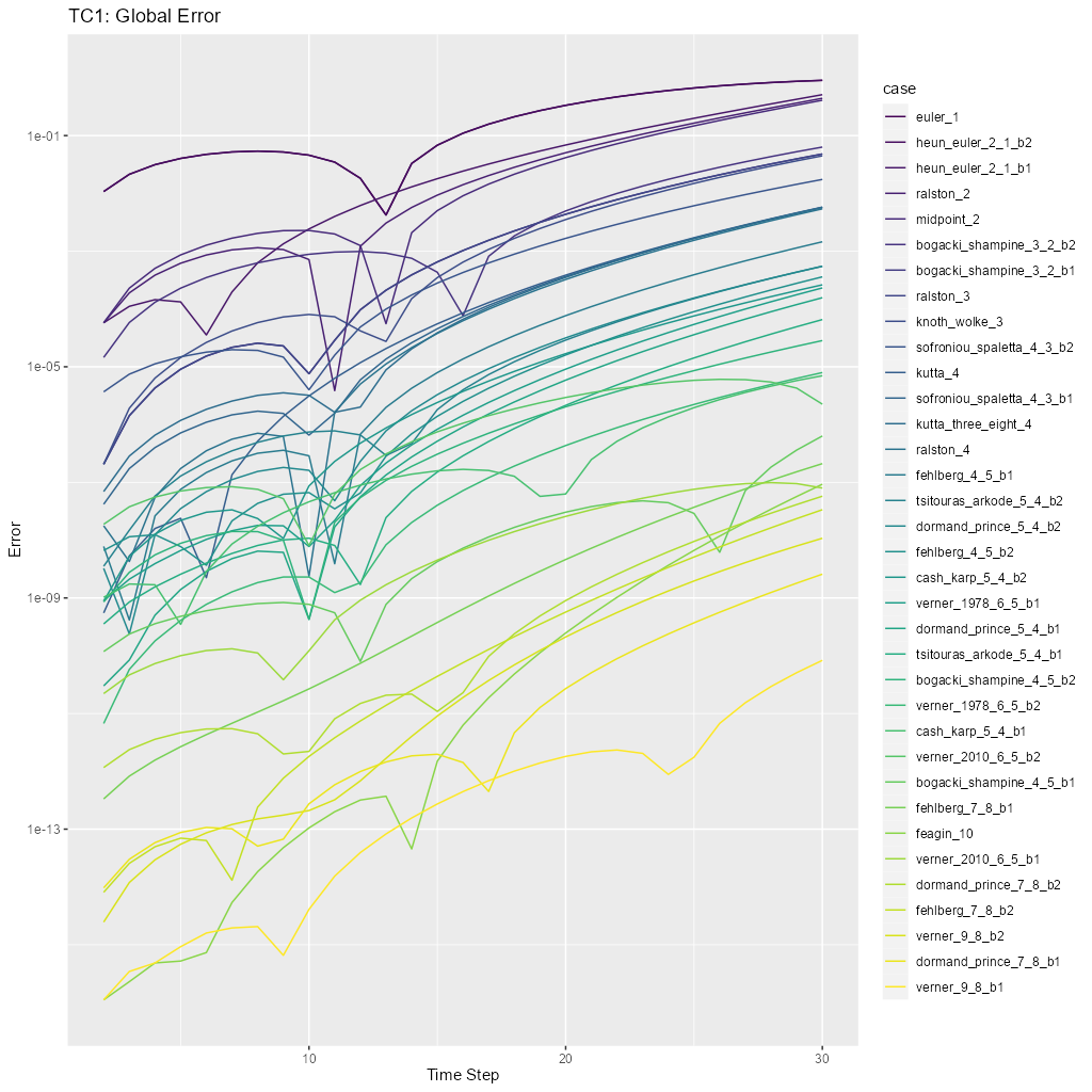
In the previous section we have some spot checks for three tableaux. In this section we have tests that verify the plausibility of the remaining methods. What do I mean by "plausibility"? I mean that we can verify that the tableaux define methods that at least seem to act like well behaved RK methods of the appropriate order.
These tests also serve as "change detection". That is to say, if I change something in the code and get different results then I may have introduced a bug.
tc1_pngThis will run the tests and display diagnostic visualizations a human can check for plausibility. Note thetc1.Rfile contains R code that may be useful in investigating these results.test_tc1This will compare the output of the tests to archived results inMRKISS/tests/data/to detect changes.
Note these tests include about 40 individual test cases each with it's own Fortran source. These tests are generated from a single seed Fortran source file
named tc1_template.f90 that is expanded into the remaining source files via the
script tc_make_make.rb. All of this is handled in the make file which will
regenerate all the test source if the template is modified.
The test equation used is:
\[ \frac{\mathrm{d}y}{\mathrm{d}t} = e^\left(-t^2\right) \]
The primary diagnostic plot is of global error:
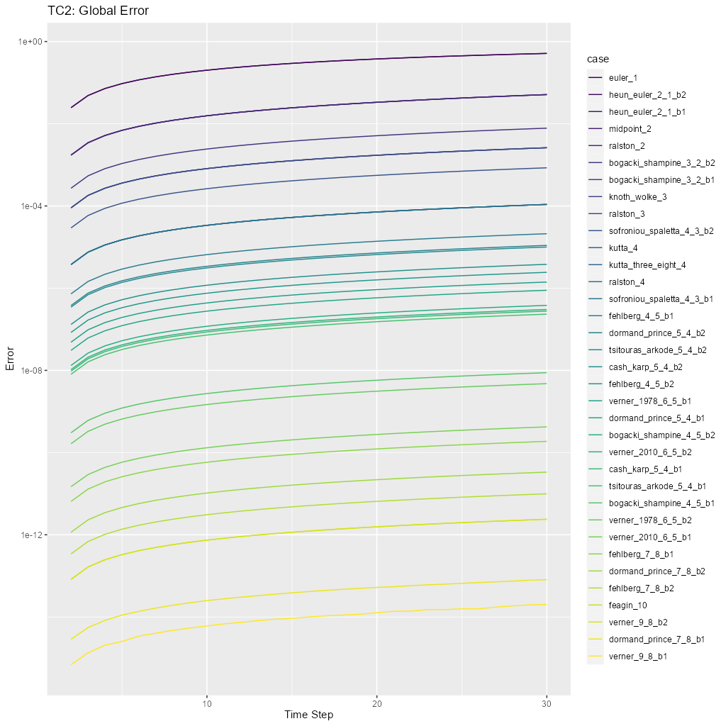
12.3. Autonomous Solvers and More Tableau Plausibility Tests
In the previous section we documented plausibility tests for the tableaux via the mrkiss_solvers_wt module. This set of tests
continues that with a new test equation:
\[ \frac{\mathrm{d}y}{\mathrm{d}t} = -2y \]
For these tests we use the autonomous solvers in the mrkiss_solvers_nt module. This source code for this module is entirely generated from
mrkiss_solvers_wt.f90 via
wt2nt.sed. So these tests also serve as a way to make sure this code gets generated and
produces reasonable results.
Like the tests in the previous section these tests also serve as "change detection". That is to say, if I change something in the code and get different results then I may have introduced a bug.
tc2_pngThis will run the tests and display diagnostic visualizations a human can check for plausibility. Note thetc2.Rfile contains R code that may be useful in investigating these results.test_tc2This will compare the output of the tests to archived results inMRKISS/tests/data/to detect changes.
Note these tests include about 40 individual test cases each with it's own Fortran source. These tests are generated from a single seed Fortran source file
named tc2_template.f90 that is expanded into the remaining source files via the
script tc_make_make.rb. All of this is handled in the make file which will
regenerate all the test source if the template is modified.
The primary diagnostic plot is of global error:
12.4. Short Stages
The step_one*(), fixed_t_steps*(), steps_condy*(), and steps_sloppy_condy*() solvers all use the b vector to determine the number of stages –
not the size of a. This allows us to use a shorter b vector cutting off trailing zero entries. This test makes sure this functionality works.
test_short_bRuns the following teststest_short_b_sub_vs_arcCompare full stage results with truncated resultstest_short_b_all_vs_subCompare with archived output inMRKISS/tests/data/.
12.5. Examples Are Tests Too
The MRKISS/examples/tdata/ directory in
MRKISS/examples/ is used to archive old output files generated from running the examples. The
makefile contains tests to run the examples and compare the results to what was
archived. These tests serve as "change detection" helping me to identify the introduction of bugs. All of these tests may be run with the tests target:
tests : test_minimal test_brusselator test_lorenz test_three_body test_step_order_vs_error
13. FAQ
13.1. What's with the name?
It's an overlapping acronym
MRKISS => MR RK KISS => Mitch Richling's Runge-Kutta Keep It Super Simple
Having such a complex name for a super simple library amuses me… Perhaps more than it should…
13.2. Why Fortran
I do most of my programming in other languages, but I really like Fortran specifically for this kind of work. It's just good at math. Especially when vectors and matrices are involved.
13.3. Why did you write another ODE solver when so many good options exist?
For a long time I have had a few annoyances related available packages:
- Sharing results and code required others to install and learn a complex software tool chain.
- Some generative art use cases drive some odd requirements that can be frustratingly difficult to do with some packages.
- Getting tools installed on new supercomputers and HPC clusters can be a challenge. It can even be annoying in the cloud.
Then one day I spent four hours trying to get my normal technical computing environment deployed to a new supercomputer with insufficient user privilege and a broken user space package manager. I wrote this library over the following weekend. ;)
In short, sometimes I just want something to work without downloading and installing gigabytes of stuff.
Oh. And I enjoy writing this kind of code..
13.4. Why don't you use package XYZ?
Don't get me wrong, I do use other packages!
One of my favorites is Julia's DifferentialEquations.jl. For bare-metal, I'm quite fond of
SUNDIALS. I also find myself using higher level tools like
R, MATLAB/Octave, and
Maple/Maxima.
13.5. What are those zotero links in the references?
Zotero is a bibliography tool. On my computer, those links take me to the Zotero application with the reference in question highlighted. This allows me to see the full bibliography entry and related documents (like personal notes, etc…).
Unfortunately they are not of much use to anyone but me.
13.6. Are high order RK methods overkill for strange attractors?
Yes. In fact, Euler's method is normally good enough for strange attractors.
13.7. I need a more comprehensive solution. Do you have advice?
My favorite is Julia's DifferentialEquations.jl. It is comprehensive, well designed, fast, and
pretty easy to use.
If you are looking for something you can call from C, C++, or Fortran then my first choice is SUNDIALS.
The ode* set of commands in MATLAB/Octave are easy to use, work well, and are extensively
documented. In addition, Octave has lsode built-in which is pretty cool.
Maple has a good selection of numerical solvers, a well designed interface, and rich ODE related graphics. It also has some of the best symbolic ODE capabilities available.
If you are doing statistics in combination with ODEs, then R is a fantastic choice.
13.8. I need something faster. Do you have advice?
All of the options listed for the question "I need a more comprehensive solution. Do you have
advice?" are faster than MRKISS. In particular Julia's
DifferentialEquations.jl and SUNDIALS.
If you are looking for something small without a lot of dependencies, then you might like Hairer's classic
codes – they are faster than MRKISS.
13.9. It seems like things are used other than Fortran. Are there really no external dependencies?
I use several tools in the development of MRKISS. In addition several of the examples use external tools to draw
graphs. None of these tools are required to compile and use the package because I have included all the generated code in the repository. Here is a summary:
- POSIX shell (
sh) - Generate
step_onefromstep_allinmrkiss_solvers_wt.f90. - Some makefile constructs for code generation, plotting, testing, etc…
- Generate
- sed
- Generate
step_onefromstep_allinmrkiss_solvers_wt.f90. - Generate
mrkiss_solvers_nt.f90frommrkiss_solvers_wt.f90.
- Generate
- ruby
- Generate code and make files for testing
- My
float_diff.rbscript, used by the tests.
- R
- Visualize output files
- GNUplot
- Visualize output files
- Maple
- Butcher tableau computations.
- nomacs
- Display images
- ImageMagick
- Process and/or convert image files
- Doxygen
- Generate API documentation
- LaTeX
- Generate logo images
- ghostscript
- Generate logo images
- rsync
- Deploy doxygen documentation to my web site
13.10. What is a "Release"? How is it different from what's on HEAD?
Releases are contained in commits with a tag that looks like this: "vYYYY-MM-DD" – i.e. an ISO 8601 format date prefixed with the letter "v". These commits differ from other commits in terms of quality control. Release commits:
- Unit tests are all successful. For information on platforms tested, see What platforms are known to work?.
- Development documentation (changelog & roadmap) are both up to date.
- Example documentation is newer than the corresponding example source.
- Doxygen documentation
- Has been generated after the most recently modified source code file.
- Has a version number that matches the tag.
- Has been deployed to by web site.
- The repository is clean.
- The manifest file
- Newer than all source code files
- Checksums match what is in repository
- It's checked into git
That said, I generally try to only push working code to github so HEAD should be reasonably safe. You can see what changes have been made on HEAD
by taking a look at the latest changelog section.
13.11. What platforms are known to work?
I have used MRKISS on a variety of platforms including:
- Various supercomputers and HPC platforms.
- Cloud hosted linux systems using various distributions: RH, SuSE, Debian, Ubuntu, & Arch.
- Physical laptop running Windows 11 using
- The MSYS2 environment
- WSL with Debian
When performing a release I test on my primary development system which changes over time. See the changelog for details.